Euler spiral

A double-end Euler spiral. The curve continues to converge to the points marked, as t tends to positive or negative infinity.

An Euler spiral is a curve whose curvature changes linearly with its curve length (the curvature of a circular curve is equal to the reciprocal of the radius). Euler spirals are also commonly referred to as spiros, clothoids, or Cornu spirals.

Euler spirals have applications to diffraction computations. They are also widely used as transition curves in railroad engineering/highway engineering for connecting and transiting the geometry between a tangent and a circular curve. A similar application is also found in photonic integrated circuits. The principle of linear variation of the curvature of the transition curve between a tangent and a circular curve defines the geometry of the Euler spiral:

Its curvature begins with zero at the straight section (the tangent) and increases linearly with its curve length.
Where the Euler spiral meets the circular curve, its curvature becomes equal to that of the latter.

Applications

Track transition curve

Animation depicting evolution of a Cornu spiral with the tangential circle with the same radius of curvature as at its tip, also known as an osculating circle (click on thumbnail to observe).

To travel along a circular path, an object needs to be subject to a centripetal acceleration (e.g.: the moon circles around the earth because of gravity; a car turns its front wheels inward to generate a centripetal force). If a vehicle traveling on a straight path were to suddenly transition to a tangential circular path, it would require centripetal acceleration suddenly switching at the tangent point from zero to the required value; this would be difficult to achieve (think of a driver instantly moving the steering wheel from straight line to turning position, and the car actually doing it), putting mechanical stress on vehicle's parts, and causing much discomfort (causing jerk).

On early railroads this instant application of lateral force was not an issue since low speeds and wide-radius curves were employed (lateral forces on the passengers and the lateral sway was small and tolerable). As speeds of rail vehicles increased over the years, it became obvious that an easement is necessary so that the centripetal acceleration increases linearly with the traveled distance. Given the expression of centripetal acceleration $V² / R$ , the obvious solution is to provide an easement curve whose curvature, $1 / R$ , increases linearly with the traveled distance. This geometry is an Euler spiral.

Unaware of the solution of the geometry by Leonhard Euler, Rankine cited the cubic curve (a polynomial curve of degree 3), which is an approximation of the Euler spiral for small angular changes in the same way that a parabola is an approximation to a circular curve.

Marie Alfred Cornu (and later some civil engineers) also solved the calculus of Euler spiral independently. Euler spirals are now widely used in rail and highway engineering for providing a transition or an easement between a tangent and a horizontal circular curve.

Optics

The Cornu spiral can be used to describe a diffraction pattern.^[1]

Integrated optics

Bends with continuously varying radius of curvature following the Euler spiral are also used to reduce losses in photonic integrated circuits, either in singlemode waveguides,^[2]^[3] to smoothen the abrupt change of curvature and coupling to radiation modes, or in multimode waveguides,^[4] in order to suppress coupling to higher order modes and ensure effective singlemode operation. A pioneering and very elegant application of the Euler spiral to waveguides had been made as early as 1957,^[5] with a hollow metal waveguide for microwaves. There the idea was to exploit the fact that a straight metal waveguide can be physically bent to naturally take a gradual bend shape resembling an Euler spiral.

Auto Racing

Motorsport author Adam Brouillard has shown the Euler spiral's use in optimizing the racing line during the corner entry portion of a turn.^[6]

Typography and digital vector drawing

Raph Levien has released Spiro as a toolkit for curve design, especially font design, in 2007^[7]^[8] under a free licence. This toolkit has been implemented quite quickly afterwards in the font design tool Fontforge and the digital vector drawing Inkscape.

Formulation

Symbols

$R$	Radius of curvature
$R_{c}$	Radius of Circular curve at the end of the spiral
$\theta$	Angle of curve from beginning of spiral (infinite $R$ ) to a particular point on the spiral.
	This can also be measured as the angle between the initial tangent and the tangent at the concerned point.
$\theta _{s}$	Angle of full spiral curve
$L,s$	Length measured along the spiral curve from its initial position
$L_{s},s_{o}$	Length of spiral curve

Derivation

The graph on the right illustrates an Euler spiral used as an easement (transition) curve between two given curves, in this case a straight line (the negative x axis) and a circle. The spiral starts at the origin in the positive x direction and gradually turns anticlockwise to osculate the circle.

The spiral is a small segment of the above double-end Euler spiral in the first quadrant.

From the definition of the curvature,

{\frac {1}{R}}={\frac {d\theta }{ds}}\propto s

i.e.

Rs={\text{constant}}=R_{c}s_{o}

{\frac {d\theta }{ds}}={\frac {s}{R_{c}s_{o}}}

We write in the format,

{\frac {d\theta }{ds}}=2a^{2}s

Where

2a^{2}={\frac {1}{R_{c}s_{o}}}

Or

a={\frac {1}{{\sqrt {2R_{c}s_{o}}}}}

Thus

\theta =(as)^{2}

Now

{\begin{aligned}x&=\int _{0}^{L}\cos \theta \,ds\\&=\int _{0}^{L}\cos \left[(as)^{2}\right]ds\end{aligned}}

If

s'=as

Then

ds={\frac {ds'}{a}}

Thus

x={\frac {1}{a}}\int _{0}^{{L'}}\cos {s}^{2}ds

{\begin{aligned}y&=\int _{0}^{L}\sin \theta \,ds\\&=\int _{0}^{L}\sin \left[(as)^{2}\right]ds\\&={\frac {1}{a}}\int _{0}^{{L'}}\sin {s}^{2}\,ds\end{aligned}}

Expansion of Fresnel integral

If a = 1, which is the case for normalized Euler curve, then the Cartesian coordinates are given by Fresnel integrals (or Euler integrals):

{\begin{aligned}C(L)&=\int _{0}^{L}\cos(s^{2})\,ds\\S(L)&=\int _{0}^{L}\sin(s^{2})\,ds\end{aligned}}

Normalization and conclusion

For a given Euler curve with:

2RL=2R_{c}L_{s}={\frac {1}{a^{2}}}

or

{\frac {1}{R}}={\frac {L}{R_{c}L_{s}}}=2a^{2}L

then

x={\frac {1}{a}}\int _{0}^{{L'}}\cos s^{2}\,ds

y={\frac {1}{a}}\int _{0}^{L'}\sin s^{2}\,ds

where $L'=aL$ and $a={\frac {1}{{\sqrt {2R_{c}L_{s}}}}}$ .

The process of obtaining solution of $(x, y)$ of an Euler spiral can thus be described as:

Map L of the original Euler spiral by multiplying with factor a to L′ of the normalized Euler spiral;
Find $(x', y')$ from the Fresnel integrals; and
Map $(x', y')$ to $(x, y)$ by scaling up (denormalize) with factor $1/a$ . Note that $1/a>1$ .

In the normalization process,

{\begin{aligned}R'_{c}&={\frac {R_{c}}{{\sqrt {2R_{c}L_{s}}}}}\\&={\sqrt {{\frac {R_{c}}{2L_{s}}}}}\\\end{aligned}}

{\begin{aligned}L'_{s}&={\frac {L_{s}}{{\sqrt {2R_{c}L_{s}}}}}\\&={\sqrt {{\frac {L_{s}}{2R_{c}}}}}\end{aligned}}

Then

{\begin{aligned}2R'_{c}L'_{s}&=2{\sqrt {{\frac {R_{c}}{2L_{s}}}}}{\sqrt {{\frac {L_{s}}{2R_{c}}}}}\\&={\tfrac {2}{2}}\\&=1\end{aligned}}

Generally the normalization reduces L' to a small value (<1) and results in good converging characteristics of the Fresnel integral manageable with only a few terms (at a price of increased numerical instability of the calculation, esp. for bigger $\theta$ values.).

Illustration

Given:

{\begin{aligned}R_{c}&=300{\mbox{m}}\\L_{s}&=100{\mbox{m}}\end{aligned}}

Then

{\begin{aligned}\theta _{s}&={\frac {L_{s}}{2R_{c}}}\\&={\frac {100}{2\times 300}}\\&=0.1667\ {\mbox{radian}}\\\end{aligned}}

And

2R_{c}L_{s}=60,000

We scale down the Euler spiral by √60,000, i.e.100√6 to normalized Euler spiral that has:

{\begin{aligned}R'_{c}={\tfrac {3}{{\sqrt {6}}}}{\mbox{m}}\\L'_{s}={\tfrac {1}{{\sqrt {6}}}}{\mbox{m}}\\\\\end{aligned}}

{\begin{aligned}2R'_{c}L'_{s}&=2\times {\tfrac {3}{{\sqrt {6}}}}\times {\tfrac {1}{{\sqrt {6}}}}\\&=1\end{aligned}}

And

{\begin{aligned}\theta _{s}&={\frac {L'_{s}}{2R'_{c}}}\\&={\frac {{\tfrac {1}{{\sqrt {6}}}}}{2\times {\tfrac {3}{{\sqrt {6}}}}}}\\&=0.1667\ {\mbox{radian}}\\\end{aligned}}

The two angles $\theta _{s}$ are the same. This thus confirms that the original and normalized Euler spirals are geometrically similar. The locus of the normalized curve can be determined from Fresnel Integral, while the locus of the original Euler spiral can be obtained by scaling back / up or denormalizing.

Other properties of normalized Euler spirals

Normalized Euler spirals can be expressed as:

x=\int _{0}^{L}\cos s^{2}ds

y=\int _{0}^{L}\sin s^{2}ds

Or expressed as power series:

x=\left.\sum _{i=0}^{\infty }{\frac {(-1)^{i}}{(2i)!}}{\frac {s^{4i+1}}{4i+1}}\right|_{0}^{L}=\sum _{i=0}^{\infty }{\frac {(-1)^{i}}{(2i)!}}{\frac {L^{4i+1}}{4i+1}}

y=\left.\sum _{i=0}^{\infty }{\frac {(-1)^{i}}{(2i+1)!}}{\frac {s^{4i+3}}{4i+3}}\right|_{0}^{L}=\sum _{i=0}^{\infty }{\frac {(-1)^{i}}{(2i+1)!}}{\frac {L^{4i+3}}{4i+3}}

The normalized Euler spiral will converge to a single point in the limit, which can be expressed as:

x^{\prime }=\lim _{L\to \infty }\int _{0}^{L}\cos(s^{2})ds={\frac {1}{2}}{\sqrt {\frac {\pi }{2}}}

y^{\prime }=\lim _{L\to \infty }\int _{0}^{L}\sin(s^{2})ds={\frac {1}{2}}{\sqrt {\frac {\pi }{2}}}

Normalized Euler spirals have the following properties:

2R_{c}L_{s}=1

\theta _{s}={\frac {L_{s}}{2R_{c}}}=L_{s}^{2}

And

\theta =\theta _{s}\cdot {\frac {L^{2}}{L_{s}^{2}}}=L^{2}

{\frac {1}{R}}={\frac {d\theta }{dL}}=2L

Note that $2R_{c}L_{s}=1$ also means $1/R_{c}=2L_{s}$ , in agreement with the last mathematical statement.

Code for producing an Euler spiral

The following SageMath code produces the second graph above. The first four lines express the Euler spiral component. Fresnel functions could not be found. Instead, the integrals of two expanded Taylor series are adopted. The remaining code expresses respectively the tangent and the circle, including the computation for the center coordinates.

var('L')
p = integral(taylor(cos(L^2), L, 0, 12), L)
q = integral(taylor(sin(L^2), L, 0, 12), L)
r1 = parametric_plot([p, q], (L, 0, 1), color = 'red')
r2 = line([(-1.0, 0), (0,0)], rgbcolor = 'blue')
x1 = p.subs(L = 1)
y1 = q.subs(L = 1)
R = 0.5
x2 = x1 - R*sin(1.0)
y2 = y1 + R*cos(1.0)
r3 = circle((x2, y2), R, rgbcolor = 'green')
show(r1 + r2 + r3, aspect_ratio = 1, axes=false)

The following is Mathematica code for the Euler spiral component (it works directly in wolframalpha.com):

ParametricPlot[{
  FresnelC[Sqrt[2/\[Pi]] t]/Sqrt[2/\[Pi]],
  FresnelS[Sqrt[2/\[Pi]] t]/Sqrt[2/\[Pi]]
}, {t, -10, 10}]

The following is Xcas code for the Euler spiral component:

plotparam([int(cos(u^2),u,0,t),int(sin(u^2),u,0,t)],t,-4,4)

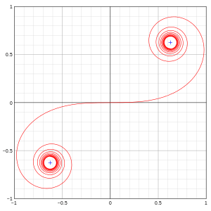
The following is SageMath code for the complete double ended Euler spiral:

s = var('s')
parametric_plot((lambda s: numerical_integral(cos(x**2),0,s)[0], lambda s: numerical_integral(sin(x**2),0,s)[0]), (-3*pi/2, 3*pi/2))

The following is JavaScript code for drawing an Euler spiral on a canvas element:

function drawEulerSpiral(canvas, T, N, scale) {
      ctx = canvas.getContext("2d");
      var dx, dy, t=0, prev = {x:0, y:0}, current;
      var dt = T/N;
      ctx.beginPath();
      while (N--) {
         dx = Math.cos(t*t) * dt;
         dy = Math.sin(t*t) * dt;
         t += dt;
         current = {
            x: prev.x + dx,
            y: prev.y + dy
         };
         ctx.lineTo(current.x*scale, current.y*scale);
         prev = current;
      }
      ctx.stroke();
}
drawEulerSpiral(document.getElementById("myCanvas"),10,10000,100)

The following is Logo (programming language) code for drawing the Euler spiral using the turtle sprite.

rt 90
repeat 720 [ fd 10 lt repcount ]

References

Notes

↑ Eugene Hecht (1998). Optics (3rd ed.). Addison-Wesley. p. 491. ISBN 0-201-30425-2.
↑ Kohtoku, M.; et al. (7 July 2005). "New Waveguide Fabrication Techniques for Next-generation PLCs" (PDF). NTT Technical Review. 3 (7): 37–41. Retrieved 24 January 2017.
↑ Li, G.; et al. (11 May 2012). "Ultralow-loss, high-density SOI optical waveguide routing for macrochip interconnects". Optics Express. 20 (11): 12035–12039. doi:10.1364/OE.20.012035. Retrieved 24 January 2017.
↑ Cherchi, M.; et al. (18 July 2013). "Dramatic size reduction of waveguide bends on a micron-scale silicon photonic platform". Optics Express. 21 (15): 17814–17823. doi:10.1364/OE.21.017814. Retrieved 24 January 2017.
↑ Unger, H.G. (September 1957). "Normal Mode Bends for Circular Electric Waves". The Bell System Technical Journal. 36 (5): 1292–1307. doi:10.1002/j.1538-7305.1957.tb01509.x. Retrieved 24 January 2017.
↑ Development, Paradigm Shift Driver; Brouillard, Adam (2016-03-18). The Perfect Corner: A Driver's Step-By-Step Guide to Finding Their Own Optimal Line Through the Physics of Racing. Paradigm Shift Motorsport Books. ISBN 9780997382426.
↑ http://levien.com/spiro/
↑ http://www.typophile.com/node/33531

Sources

External links

This article is issued from Wikipedia. The text is licensed under Creative Commons - Attribution - Sharealike. Additional terms may apply for the media files.

[Hecht-1] Eugene Hecht (1998). Optics (3rd ed.). Addison-Wesley. p. 491. ISBN 0-201-30425-2.

[2] Kohtoku, M.; et al. (7 July 2005). "New Waveguide Fabrication Techniques for Next-generation PLCs" (PDF). NTT Technical Review. 3 (7): 37–41. Retrieved 24 January 2017.

[3] Li, G.; et al. (11 May 2012). "Ultralow-loss, high-density SOI optical waveguide routing for macrochip interconnects". Optics Express. 20 (11): 12035–12039. doi:10.1364/OE.20.012035. Retrieved 24 January 2017.

[4] Cherchi, M.; et al. (18 July 2013). "Dramatic size reduction of waveguide bends on a micron-scale silicon photonic platform". Optics Express. 21 (15): 17814–17823. doi:10.1364/OE.21.017814. Retrieved 24 January 2017.

[5] Unger, H.G. (September 1957). "Normal Mode Bends for Circular Electric Waves". The Bell System Technical Journal. 36 (5): 1292–1307. doi:10.1002/j.1538-7305.1957.tb01509.x. Retrieved 24 January 2017.

[6] Development, Paradigm Shift Driver; Brouillard, Adam (2016-03-18). The Perfect Corner: A Driver's Step-By-Step Guide to Finding Their Own Optimal Line Through the Physics of Racing. Paradigm Shift Motorsport Books. ISBN 9780997382426.

[7] ttp://levien.com/spiro/

[8] ttp://www.typophile.com/node/33531

Spirals, curves and helices
Curves	Algebraic Curvature Gallery List Topics
Helices	3₁₀ Alpha Angle Beta Boerdijk–Coxeter Double Antenna Hemi Pi Polyproline Super Symmetry Triple Collagen
Spirals	Archimedean Cotes's Epispiral Hyperbolic Poinsot's Euler Fermat's Golden Logarithmic On Spirals Theodorus

Euler spiral

Applications

Track transition curve

Optics

Integrated optics

Auto Racing

Typography and digital vector drawing

Formulation

Symbols

Expansion of Fresnel integral

Normalization and conclusion

Illustration

Other properties of normalized Euler spirals

Code for producing an Euler spiral

See also

References

Further reading

External links