Difference in differences

Difference in differences (DID^[1] or DD^[2]) is a statistical technique used in econometrics and quantitative research in the social sciences that attempts to mimic an experimental research design using observational study data, by studying the differential effect of a treatment on a 'treatment group' versus a 'control group' in a natural experiment.^[3] It calculates the effect of a treatment (i.e., an explanatory variable or an independent variable) on an outcome (i.e., a response variable or dependent variable) by comparing the average change over time in the outcome variable for the treatment group, compared to the average change over time for the control group. Although it is intended to mitigate the effects of extraneous factors and selection bias, depending on how the treatment group is chosen, this method may still be subject to certain biases (e.g., mean regression, reverse causality and omitted variable bias).

In contrast to a time-series estimate of the treatment effect on subjects (which analyzes differences over time) or a cross-section estimate of the treatment effect (which measures the difference between treatment and control groups), difference in differences uses panel data to measure the differences, between the treatment and control group, of the changes in the outcome variable that occur over time.

General definition

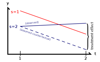
Difference in differences requires data measured from a treatment group and a control group at two or more different time periods, specifically at least one time period before "treatment" and at least one time period after "treatment." In the example pictured, the outcome in the treatment group is represented by the line P and the outcome in the control group is represented by the line S. The outcome (dependent) variable in both groups are measured at time period 1, before either group has received the treatment (i.e., the independent or explanatory variable), represented by the points P₁ and S₁. The treatment group then receives or experiences the treatment and both groups are again measured at time period 2. Not all of the difference between the treatment and control groups at time period 2 (that is, the difference between P₂ and S₂) can be explained as being an effect of the treatment, because the treatment group and control group did not start out at the same point at time period 1. DID therefore calculates the "normal" difference in the outcome variable between the two groups (the difference that would still exist if neither group experienced the treatment), represented by the dotted line Q. (Notice that the slope from P₁ to Q is the same as the slope from S₁ to S₂.) The treatment effect is the difference between the observed outcome and the "normal" outcome (the difference between P₂ and Q).

Formal definition

Consider the model

y_{it}~=~\gamma _{s(i)}+\lambda _{t}+\delta I(s(i){\text{ is the treatment group, }}t{\text{ is in the after period}})+\varepsilon _{it}

where $y_{{it}}$ is the dependent variable for individual $i$ and $t$ , $s(i)$ is the group to which $i$ belongs, and $I(\dots )$ is short-hand for the dummy variable equal to 1 when the event described in $(\dots )$ is true, and 0 otherwise. In the plot of time versus $Y$ by group, $\gamma_s$ is the vertical intercept for the graph for $s$ , and $\lambda_t$ is the time trend shared by both group according to the parallel trend assumption. $\delta$ is the treatment effect, and $\varepsilon _{it}$ is the residual term.

Let's consider the average of the dependent variable and dummy indicators by group and time:

{\begin{aligned}n_{s}&={\text{ number of individuals in group }}s\\{\overline {y}}_{st}&={\frac {1}{n_{s}}}\sum _{i=1}^{n}y_{it}\ I(s(i)~=~s),\\{\overline {\gamma }}_{s}&={\frac {1}{n_{s}}}\sum _{i=1}^{n}\gamma _{s}(i)\ I(s(i)~=~s)~=~\gamma _{s},\\{\overline {\lambda }}_{st}&={\frac {1}{n_{s}}}\sum _{i=1}^{n}\lambda _{t}\ I(s(i)~=~s)~=~\lambda _{t},\\D_{st}&={\frac {1}{n_{s}}}\sum _{i=1}^{n}I(s(i)~=~{\text{ treatment, }}t{\text{ in after period}})\ I(s(i)~=~s)~=~I(s~=~{\text{ treatment, }}t{\text{ in after period}}),\\{\overline {\varepsilon }}_{st}&={\frac {1}{n_{s}}}\sum _{i=1}^{n}\varepsilon _{it}\ I(s(i)~=~s),\end{aligned}}

and suppose for simplicity that $s=1,2$ and $t=1,2$ . Note that $D_{{st}}$ is not random; it just encodes how the groups and the periods are labeled. Then

{\begin{aligned}&({\overline {y}}_{11}-{\overline {y}}_{12})-({\overline {y}}_{21}-{\overline {y}}_{22})\\[6pt]={}&{\big [}(\gamma _{1}+\lambda _{1}+\delta D_{11}+{\overline {\varepsilon }}_{11})-(\gamma _{1}+\lambda _{2}+\delta D_{12}+{\overline {\varepsilon }}_{12}){\big ]}\\&\qquad {}-{\big [}(\gamma _{2}+\lambda _{1}+\delta D_{21}+{\overline {\varepsilon }}_{21})-(\gamma _{2}+\lambda _{2}+\delta D_{22}+{\overline {\varepsilon }}_{22}){\big ]}\\[6pt]={}&\delta (D_{11}-D_{12})+\delta (D_{22}-D_{21})+{\overline {\varepsilon }}_{11}-{\overline {\varepsilon }}_{12}+{\overline {\varepsilon }}_{22}-{\overline {\varepsilon }}_{21}.\end{aligned}}

The strict exogeneity assumption then implies that

\operatorname {E} \left[({\overline {y}}_{11}-{\overline {y}}_{12})-({\overline {y}}_{21}-{\overline {y}}_{22})\right]~=~\delta (D_{11}-D_{12})+\delta (D_{22}-D_{21}).

Without loss of generality, assume that $s=2$ is the treatment group, and $t = 2$ is the after period, then $D_{{22}}=1$ and $D_{{11}}=D_{{12}}=D_{{21}}=0$ , giving the DID estimator

{\hat {\delta }}~=~({\overline {y}}_{11}-{\overline {y}}_{12})-({\overline {y}}_{21}-{\overline {y}}_{22}),

which can be interpreted as the treatment effect of the treatment indicated by $D_{{st}}$ . Below it is shown how this estimator can be read as a coefficient in an ordinary least squares regression. The model described in this section is over-parametrized; to remedy that, one of the coefficients for the dummy variables can be set to 0, for example, we may set $\gamma _{1}=0$ .

Assumptions

Illustration of the parallel trend assumption

All the assumptions of the OLS model apply equally to DID. In addition, DID requires a parallel trend assumption. The parallel trend assumption says that $\lambda _{2}-\lambda _{1}$ are the same in both $s=1$ and $s=2$ . Given that the formal definition above accurately represents reality, this assumption automatically holds. However, a model with $\lambda _{{st}}~:~\lambda _{{22}}-\lambda _{{21}}\neq \lambda _{{12}}-\lambda _{{11}}$ may well be more realistic.

As illustrated to the right, the treatment effect is the difference between the observed value of y and what the value of y would have been with parallel trends, had there been no treatment. The Achilles' heel of DID is when something other than the treatment changes in one group but not the other at the same time as the treatment, implying a violation of the parallel trend assumption.

To guarantee the accuracy of the DID estimate, the composition of individuals of the two groups is assumed to remain unchanged over time. When using a DID model, various issues that may compromise the results, such as autocorrelation and Ashenfelter dips, must be considered and dealt with.

Implementation

The DID method can be implemented according to the table below, where the lower right cell is the DID estimator.

$y_{{st}}$	$s=2$	$s=1$	Difference
$t=2$	$y_{{22}}$	$y_{{12}}$	$y_{{12}}-y_{{22}}$
$t=1$	$y_{{21}}$	$y_{{11}}$	$y_{{11}}-y_{{21}}$
Change	$y_{{21}}-y_{{22}}$	$y_{{11}}-y_{{12}}$	$(y_{{11}}-y_{{21}})-(y_{{12}}-y_{{22}})$

Running a regression analysis gives the same result. Consider the OLS model

y~=~\beta _{0}+\beta _{1}T+\beta _{2}S+\beta _{3}(T\cdot S)+\varepsilon

where $T$ is a dummy variable for the period, equal to $1$ when $t=2$ , and $S$ is a dummy variable for group membership, equal to $1$ when $s=2$ . The composite variable $(T\cdot S)$ is a dummy variable indicating when $S=T=1$ . Although it is not shown rigorously here, this is a proper parametrization of the model formal definition, furthermore, it turns out that the group and period averages in that section relate to the model parameter estimates as follows

{\begin{aligned}{\hat {\beta }}_{0}&={\widehat {E}}(y\mid T=0,~S=0)\\[8pt]{\hat {\beta }}_{1}&={\widehat {E}}(y\mid T=1,~S=0)-{\widehat {E}}(y\mid T=0,~S=0)\\[8pt]{\hat {\beta }}_{2}&={\widehat {E}}(y\mid T=0,~S=1)-{\widehat {E}}(y\mid T=0,~S=0)\\[8pt]{\hat {\beta }}_{3}&={\big [}{\widehat {E}}(y\mid T=1,~S=1)-{\widehat {E}}(y\mid T=0,~S=1){\big ]}\\&\qquad {}-{\big [}{\widehat {E}}(y\mid T=1,~S=0)-{\widehat {E}}(y\mid T=0,~S=0){\big ]},\end{aligned}}

where ${\widehat {E}}(\dots \mid \dots )$ stands for conditional averages computed on the sample, for example, $T=1$ is the indicator for the after period, $S=0$ is an indicator for the control group. To see the relation between this notation and the previous section, consider as above only one observation per time period for each group, then

{\begin{aligned}{\widehat {E}}(y\mid T=1,~S=0)&={\widehat {E}}(y\mid {\text{ after period, control}})\\[3pt]\\&={\frac {{\widehat {E}}(y\ I({\text{ after period, control}}))}{{\widehat {P}}({\text{ after period, control}})}}\\[3pt]\\&={\frac {\sum _{i=1}^{n}y_{i,{\text{after}}}I(i{\text{ in control}})}{n_{\text{control}}}}={\overline {y}}_{\text{control, after}}\\[3pt]\\&={\overline {y}}_{\text{12}}\end{aligned}}

and so on for other values of $T$ and $S$ , which is equivalent to

{\hat {\beta }}_{3}~=~(y_{11}-y_{21})-(y_{12}-y_{22}).

But this is the expression for the treatment effect that was given in the formal definition and in the above table.

Card and Krueger (1994) example

Consider one of the most famous DID studies, the Card and Krueger article on minimum wage in New Jersey, published in 1994.^[4] Card and Krueger compared employment in the fast food sector in New Jersey and in Pennsylvania, in February 1992 and in November 1992, after New Jersey's minimum wage rose from $4.25 to $5.05 in April 1992. Observing a change in employment in New Jersey only, before and after the treatment, would fail to control for omitted variables such as weather and macroeconomic conditions of the region. By including Pennsylvania as a control in a difference-in-differences model, any bias caused by variables common to New Jersey and Pennsylvania is implicitly controlled for, even when these variables are unobserved. Assuming that New Jersey and Pennsylvania have parallel trends over time, Pennsylvania's change in employment can be interpreted as the change New Jersey would have experienced, had they not increased the minimum wage, and vice versa. The evidence suggested that the increased minimum wage did not induce an increase in unemployment in New Jersey, as standard economic theory would suggest. The table below shows Card & Krueger's estimates of the treatment effect on employment, measured as FTEs (or full-time equivalents). Keeping in mind that the finding is controversial, Card and Krueger estimate that the $0.80 minimum wage increase in New Jersey led to a 2.75 FTE increase in employment.

	New Jersey	Pennsylvania	Difference
February	20.44	23.33	−2.89
November	21.03	21.17	−0.14
Change	0.59	−2.16	2.75

References

↑ Abadie, A. (2005). "Semiparametric difference-in-differences estimators". Review of Economic Studies. 72 (1): 1–19. doi:10.1111/0034-6527.00321.
↑ Bertrand, M.; Duflo, E.; Mullainathan, S. (2004). "How Much Should We Trust Differences-in-Differences Estimates?". Quarterly Journal of Economics. 119 (1): 249–275. doi:10.1162/003355304772839588.
↑ Angrist, J. D.; Pischke, J. S. (2008). Mostly Harmless Econometrics: An Empiricist's Companion. Princeton University Press. pp. 227–243. ISBN 978-0-691-12034-8.
↑ Card, David; Krueger, Alan B. (1994). "Minimum Wages and Employment: A Case Study of the Fast-Food Industry in New Jersey and Pennsylvania". American Economic Review. 84 (4): 772–793. JSTOR 2118030.

External links

Difference in Difference Estimation, Healthcare Economist website

This article is issued from Wikipedia. The text is licensed under Creative Commons - Attribution - Sharealike. Additional terms may apply for the media files.

[1] Abadie, A. (2005). "Semiparametric difference-in-differences estimators". Review of Economic Studies. 72 (1): 1–19. doi:10.1111/0034-6527.00321.

[Bertrand-2] Bertrand, M.; Duflo, E.; Mullainathan, S. (2004). "How Much Should We Trust Differences-in-Differences Estimates?". Quarterly Journal of Economics. 119 (1): 249–275. doi:10.1162/003355304772839588.

[3] Angrist, J. D.; Pischke, J. S. (2008). Mostly Harmless Econometrics: An Empiricist's Companion. Princeton University Press. pp. 227–243. ISBN 978-0-691-12034-8.

[4] Card, David; Krueger, Alan B. (1994). "Minimum Wages and Employment: A Case Study of the Fast-Food Industry in New Jersey and Pennsylvania". American Economic Review. 84 (4): 772–793. JSTOR 2118030.