Density of states

In solid state physics and condensed matter physics, the density of states (DOS) of a system describes the number of states per an interval of energy at each energy level available to be occupied. It is mathematically represented by a density distribution and it is generally an average over the space and time domains of the various states occupied by the system. A high DOS at a specific energy level means that there are many states available for occupation. A DOS of zero means that no states can be occupied at that energy level. The DOS is usually represented by one of the symbols g, ρ, D, n, or N.

Generally, the density of the states of matter is continuous. In isolated systems however, like atoms or molecules in the gas phase, the density distribution is discrete like a spectral density.

Local variations, most often due to distortions of the original system, are often called local density of states (LDOS). If the DOS of an undisturbed system is zero, the LDOS can locally be non-zero due to the presence of a local potential.

Introduction

In quantum mechanical (QM) systems, waves, or wave-like particles, can occupy modes or states with wavelengths and propagation directions dictated by the system. For example, in some systems, the interatomic spacing and the atomic charge of a material could allow only electrons of certain wavelengths to exist. In other systems, the crystalline structure of a material could allow waves to propagate in one direction, while suppressing wave propagation in another direction. Often, only specific states are permitted. Thus, it can happen that many states are available for occupation at a specific energy level, while no states are available at other energy levels .

For example, the density of states of electrons at the bandedge between the conduction band and the valence band in a semiconductor is shown in orange in Fig. 4 (in the subsequent section " Density of states and distribution functions"). For an electron in the conduction band, an increase of the electron energy causes more states to become available for occupation. Alternatively, the density of state is discontinuous for an interval of energy, which means that there are no states available for electrons to occupy within the bandgap of the material. This also means that an electron at the conduction band edge must lose at least the bandgap energy of the material in order to transition to another state in the valence band.

Depending on the QM system, the density of states can be calculated for electrons, photons, or phonons, and can be given as a function of either energy or the wave vector k. To convert between the DOS as a function of the energy and the DOS as a function of the wave vector, the system-specific energy dispersion relation between E and k must be known.

In general, the topological properties of the system have a major impact on the properties of the density of states. The most well-known systems, like neutronium in neutron stars and free electron gases in metals (examples of degenerate matter and a Fermi gas), have a 3-dimensional Euclidean topology. Less familiar systems, like 2-dimensional electron gases (2DEG) in graphite layers and the quantum Hall effect system in MOSFET type devices, have a 2-dimensional Euclidean topology. Even less familiar are carbon nanotubes, the quantum wire and Luttinger liquid with their 1-dimensional topologies. Systems with 1D and 2D topologies are likely to become more common, assuming developments in nanotechnology and materials science proceed.

Definition

In general the density of states, related to volume V and N countable energy levels, is defined by:

D(E)={\frac {1}{V}}\cdot \sum _{i=1}^{N}\delta \left(E-E\left({\vec {k}}_{i}\right)\right).

Using $(\Delta k)^{d}=\left({\frac {2\pi }{L}}\right)^{d}$ (the smallest allowed change of $k$ for a particle in a box of dimension $d$ and length $L$ ) under the limit $L\to \infty$ , one derives the volume-related density of states for continuous energy levels

D(E):=\int _{\mathbb {R} ^{d}}{\frac {\mathrm {d} ^{d}k}{(2\pi )^{d}}}\cdot \delta \left(E-E\left({\vec {k}}\right)\right).

With $d$ of the spatial dimension of the considered system and $k$ the wave vector.

Equivalently, the density of states can also be understood as the derivative of the microcanonical partition function $Z_{m}(E)$ with respect to the energy:

D(E)={\frac {1}{V}}\cdot {\frac {\mathrm {d} Z_{m}(E)}{\mathrm {d} E}}

The number of states with energy $E'$ (degree of degeneracy) is given by:

g\left(E'\right)=\lim _{\Delta E\to 0}\int _{E'}^{E'+\Delta E}D(E)\mathrm {d} E=\lim _{\Delta E\to 0}D\left(E'\right)\Delta E,

where the last equality only applies when the mean value theorem for integrals is valid.

Symmetry and density of states

First Brillouin zone of the FCC lattice, a truncated octahedron, showing symmetry labels for high symmetry lines and points

There is a large variety of systems and types of states for which DOS calculations can be done.

Some condensed matter systems possess a symmetry of its structure on its microscopic scale which simplifies calculations of its density of states. In spherically symmetric systems, the integrals of function are one-dimensional because all variables in the calculation depend only on the radial parameter of the dispersion relation. Fluids, glasses or amorphous solids are example of a symmetric system whose dispersion relations has a rotational symmetry.

Octahedron.

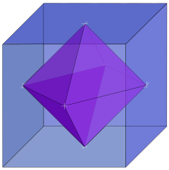
Measurements on powders or polycrystalline samples require evaluation and calculation functions and integrals over the whole domain, most often a Brillouin zone, of the dispersion relations of the system of interest. Sometimes the symmetry of the system is high, which causes the shape of the functions describing the dispersion relations of the system to appear many times over the whole domain of the dispersion relation. In such cases the effort to calculate the DOS can be reduced by a great amount when the calculation is limited to a reduced zone or fundamental domain.^[1] The Brillouin zone of the FCC lattice in the figure on the right has the 48 fold symmetry of the point group O_h with full octahedral symmetry. This means that the integration over the whole domain of the Brillouin zone can be reduced to a 48-th part of the whole Brillouin zone. As a crystal structure periodic table shows, there are many elements with a FCC crystal structure, like Diamond, Silicon and Platinum and their Brillouin zones and dispersion relations have this 48 fold symmetry. Two other familiar crystal structures are the BCC and HCP structures with cubic and hexagonal lattices, respectively. The BCC structure has the 24 fold pyritohedral symmetry of the point group T_h. The HCP structure has the 12 fold prismatic dihedral symmetry of the point group D_3h. A complete list of symmetry properties of a point group can be found in point group character tables.

In general it is easier to calculate a DOS when the symmetry of the system is higher and the number of topological dimensions of the dispersion relation is lower. The DOS of dispersion relations with rotational symmetry can often be calculated analytically. This is fortunate, since many materials of practical interest, such as steel and silicon, have high symmetry.

In anisotropic condensed matter systems such as a single crystal of a compound, the density of states could be different in one crystallographic direction than in another. These causes the anisotropic density of states to be more difficult to visualize, and might require methods such as calculating the DOS for particular points or directions only, or calculating the projected density of states (PDOS) to a particular crystal orientation.

k-space topologies

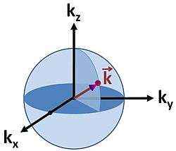
Figure 1: Spherical surface in k-space for electrons in three dimensions.

The density of states is dependent upon the dimensional limits of the object itself. In a system described by three orthogonal parameters (3 Dimension), the units of DOS is Energy⁻¹Volume⁻¹ , in a two dimensional system, the units of DOS is Energy⁻¹Area⁻¹ , in a one dimensional system, the units of DOS is Energy⁻¹Length⁻¹. It is important to note that the volume being referenced is the volume of k-space; the space enclosed by the constant energy surface of the system derived through a dispersion relation that relates E to k. An example of a 3-dimensional k-space is given in Fig. 1. It can be seen that the dimensionality of the system itself will confine the momentum of particles inside the system.

Density of wave vector states (sphere)

The calculation for DOS starts by counting the N allowed states at a certain k that are contained within [k, k + dk] inside the volume of the system. This is done by differentiating the whole k-space volume $\Omega _{n,k}$ in n-dimensions at an arbitrary k, with respect to k. The volume, area or length in 3, 2 or 1-dimensional spherical k-spaces are expressed by

\Omega _{n}(k)=c_{n}k^{n}

for a n-dimensional k-space with the topologically determined constants

c_{1}=2,\ c_{2}=\pi ,\ c_{3}={\frac {4\pi }{3}}

for linear, disk and spherical symmetrical shaped functions in 1, 2 and 3-dimensional Euclidean k-spaces respectively.

According to this scheme, the density of wave vector states N is, through differentiating $\Omega _{n,k}$ with respect to k, expressed by

N_{n}(k)={\frac {{\rm {d}}\Omega _{n}(k)}{{\rm {d}}k}}=n\;c_{n}\;k^{n-1}

The 1, 2 and 3-dimensional density of wave vector states for a line, disk, or sphere are explicitly written as

{\begin{aligned}N_{1}(k)&=2\\N_{2}(k)&=2\pi k\\N_{3}(k)&=4\pi k^{2}\end{aligned}}

One state is large enough to contain particles having wavelength λ. The wavelength is related to k through the relationship.

k={\frac {2\pi }{\lambda }}

In a quantum system the length of λ will depend on a characteristic spacing of the system L that is confining the particles. Finally the density of states N is multiplied by a factor $s/V_{k}$ , where s is a constant degeneracy factor that accounts for internal degrees of freedom due to such physical phenomena as spin or polarization. If no such phenomenon is present then $s=1$ . V_k is the volume in k-space whose wavevectors are smaller than the smallest possible wavevectors decided by the characteristic spacing of the system.

Density of energy states

To finish the calculation for DOS find the number of states per unit sample volume at an energy $E$ inside an interval $[E,E+dE]$ . The general form of DOS of a system is given as

D_{n}\left(E\right)={\frac {{\rm {d}}\Omega _{n}(E)}{{\rm {d}}E}}

The scheme sketched so far only applies to monotonically rising and spherically symmetric dispersion relations. In general the dispersion relation $E(k)$ is not spherically symmetric and in many cases it isn't continuously rising either. To express D as a function of E the inverse of the dispersion relation $E(k)$ has to be substituted into the expression of $\Omega _{n}(k)$ as a function of k to get the expression of $\Omega _{n}(E)$ as a function of the energy. If the dispersion relation is not spherically symmetric or continuously rising and can't be inverted easily then in most cases the DOS has to be calculated numerically. More detailed derivations are available.^[2]^[3]

Dispersion relations

The dispersion relation for electrons in a solid is given by the electronic band structure.

The kinetic energy of a particle depends on the magnitude and direction of the wave vector k, the properties of the particle and the environment in which the particle is moving. For example, the kinetic energy of an electron in a Fermi gas is given by

E=E_{0}+{\frac {\left(\hbar k\right)^{2}}{2m}}\ ,

where m is the electron mass. The dispersion relation is a spherically symmetric parabola and it is continuously rising so the DOS can be calculated easily.

Figure 2: Monatomic chain phonon dispersion relation

For longitudinal phonons in a string of atoms the dispersion relation of the kinetic energy in a 1-dimensional k-space, as shown in Figure 2, is given by

E=2\hbar \omega _{0}\left|\sin \left({\frac {ka}{2}}\right)\right|

where $\omega _{0}={\sqrt {k_{F}/m}}$ is the oscillator frequency, $m$ the mass of the atoms, $k_{F}$ the inter-atomic force constant and $a$ inter-atomic spacing. For small values of $k\ll \pi /a$ the dispersion relation is rather linear:

E=\hbar \omega _{0}ka

When $k\approx \pi /a$ the energy is

E=2\hbar \omega _{0}\left|\cos \left({\frac {\pi -ka}{2}}\right)\right|

With the transformation $q=k-\pi /a$ and small $q$ this relation can be transformed to

E=2\hbar \omega _{0}\left[1-\left({\frac {qa}{2}}\right)^{2}\right]

Isotropic dispersion relations

The two examples mentioned here can be expressed like

E=E_{0}+c_{k}k^{p}

This is a kind of dispersion relation because it interrelates two wave properties and it is isotropic because only the length and not the direction of the wave vector appears in the expression. The magnitude of the wave vector is related to the energy as:

k=\left({\frac {E-E_{0}}{c_{k}}}\right)^{\frac {1}{p}}\ ,

Accordingly, the volume of n-dimensional k-space containing wave vectors smaller than k is:

\Omega _{n}(k)=c_{n}k^{n}

Substitution of the isotropic energy relation gives the volume of occupied states

\Omega _{n}(E)={\frac {c_{n}}{{c_{k}}^{\frac {n}{p}}}}\left(E-E_{0}\right)^{\frac {n}{p}}\ ,

Differentiating this volume with respect to the energy gives an expression for the DOS of the isotropic dispersion relation

D_{n}\left(E\right)={\frac {d}{dE}}\Omega _{n}(E)={\frac {nc_{n}}{p{c_{k}}^{\frac {n}{p}}}}\left(E-E_{0}\right)^{{\frac {n}{p}}-1}

Parabolic dispersion

Figure 3: Free-electron DOS in 3-dimensional k-space

In the case of a parabolic dispersion relation (p = 2), such as applies to free electrons in a Fermi gas, the resulting density of states, $D_{n}\left(E\right)$ , for electrons in a n-dimensional systems is

{\begin{aligned}D_{1}\left(E\right)&={\frac {1}{\sqrt {c_{k}\left(E-E_{0}\right)}}}\\D_{2}\left(E\right)&={\frac {\pi }{c_{k}}}\\D_{3}\left(E\right)&=2\pi {\sqrt {\frac {E-E_{0}}{c_{k}^{3}}}}\ .\end{aligned}}

for $E>E_{0}$ , with $D(E)=0$ for $E<E_{0}$ .

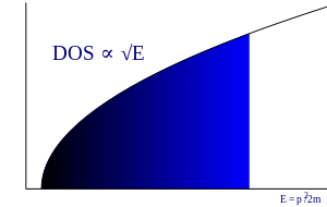
In 1-dimensional systems the DOS diverges at the bottom of the band as $E$ drops to $E_{0}$ . In 2-dimensional systems the DOS turns out to be independent of $E$ . Finally for 3-dimensional systems the DOS rises as the square root of the energy.^[4]

Including the prefactor $s/V_{k}$ , the expression for the 3D DOS is

N(E)={\frac {V}{2\pi ^{2}}}\left({\frac {2m}{\hbar ^{2}}}\right)^{\frac {3}{2}}{\sqrt {E-E_{0}}}

,

where $V$ is the total volume, and $N(E-E_{0})$ includes the 2-fold spin degeneracy.

Linear dispersion

In the case of a linear relation (p = 1), such as applies to photons, acoustic phonons, or to some special kinds of electronic bands in a solid, the DOS in 1, 2 and 3 dimensional systems is related to the energy as:

{\begin{aligned}D_{1}\left(E\right)&={\frac {1}{c_{k}}}\\D_{2}\left(E\right)&={\frac {2\pi }{c_{k}^{2}}}\left(E-E_{0}\right)\\D_{3}\left(E\right)&={\frac {4\pi }{c_{k}^{3}}}\left(E-E_{0}\right)^{2}\end{aligned}}

Distribution functions

The density of states plays an important role in the kinetic theory of solids. The product of the density of states and the probability distribution function is the number of occupied states per unit volume at a given energy for a system in thermal equilibrium. This value is widely used to investigate various physical properties of matter. The following are examples, using two common distribution functions, of how applying a distribution function to the density of states can give rise to physical properties.

Figure 4: The Fermi-Dirac probability distribution, density of states, and their product for a semiconductor. The lower green lobe depicts hole energy, and thus uses

f(-x)

as the distribution function.

Fermi–Dirac statistics: The Fermi–Dirac probability distribution function, Fig. 4, is used to find the probability that a fermion occupies a specific quantum state in a system at thermal equilibrium. Fermions are particles which obey the Pauli exclusion principle (e.g. electrons, protons, neutrons). The distribution function can be written as

f_{\mathrm {FD} }(E)={\frac {1}{\exp \left({\frac {E-\mu }{k_{\mathrm {B} }T}}\right)+1}}

$\mu$ is the chemical potential (also denoted as E_F and called the Fermi level when T=0), $k_{\mathrm {B} }$ is the Boltzmann constant, and $T$ is temperature. Fig. 4 illustrates how the product of the Fermi-Dirac distribution function and the three-dimensional density of states for a semiconductor can give insight to physical properties such as carrier concentration and Energy band gaps.

Bose–Einstein statistics: The Bose–Einstein probability distribution function is used to find the probability that a boson occupies a specific quantum state in a system at thermal equilibrium. Bosons are particles which do not obey the Pauli exclusion principle (e.g. phonons and photons). The distribution function can be written as

f_{\mathrm {BE} }(E)={\frac {1}{\exp \left({\frac {E-\mu }{k_{B}T}}\right)-1}}

From these two distributions it is possible to calculate properties such as the internal energy $U$ , the number of particles $n$ , specific heat capacity $C$ , and thermal conductivity $k$ . The relationships between these properties and the product of the density of states and the probability distribution, denoting the density of states by $g(E)$ instead of $D(E)$ , are given by

{\begin{aligned}U&=\int E\,f(E)\,g(E)\,{\rm {d}}E\\n&=\int f(E)\,g(E)\,{\rm {d}}E\\C&={\frac {\partial }{\partial T}}\int E\,f(E)\,g(E)\,{\rm {d}}E\\k&={\frac {1}{d}}{\frac {\partial }{\partial T}}\int Ef(E)\,g(E)\,\nu (E)\,\Lambda (E)\,{\rm {d}}E\end{aligned}}

$d$ is dimensionality, $\nu$ is sound velocity and $\Lambda$ is mean free path.

Applications

The density of states appears in many areas of physics, and helps to explain a number of quantum mechanical phenomena.

Quantization

Calculating the density of states for small structures shows that the distribution of electrons changes as dimensionality is reduced. For quantum wires, the DOS for certain energies actually becomes higher than the DOS for bulk semiconductors, and for quantum dots the electrons become quantized to certain energies.

Photonic crystals

The photon density of states can be manipulated by using periodic structures with length scales on the order of the wavelength of light. Some structures can completely inhibit the propagation of light of certain colors (energies), creating a photonic bandgap: the DOS is zero for those photon energies. Other structures can inhibit the propagation of light only in certain directions to create mirrors, waveguides, and cavities. Such periodic structures are known as photonic crystals. In nanostructured media the concept of Local density of states (LDOS) is often more relevant than that of DOS, as the DOS varies considerably from point to point.

Computational calculation

Interesting systems are in general complex, for instance compounds, biomolecules, polymers, etc. Because of the complexity of these systems the analytical calculation of the density of states is in most of the cases impossible. Computer simulations offer a set of algorithms to evaluate the density of states with a high accuracy. One of these algorithms is called the Wang and Landau algorithm.^[5]

Within the Wang and Landau scheme any previous knowledge of the density of states is required. One proceeds as follows: the cost function (for example the energy) of the system is discretized. Each time the bin i is reached one updates a histogram for the density of states, $g(i)$ , by

g(i)\rightarrow g(i)+f

where f is called the modification factor. As soon as each bin in the histogram is visited a certain number of times (10-15), the modification factor is reduced by some criterion, for instance,

f_{n+1}\rightarrow {\frac {1}{2}}f_{n}

where n denotes the n-th update step. The simulation finishes when the modification factor is less than a certain threshold, for instance $f_{n}<10^{-8}$ .

The Wang and Landau algorithm has some advantages over other common algorithms such as multicanonical simulations and parallel tempering. For example, the density of states is obtained as the main product of the simulation. Additionally, Wang and Landau simulations are completely independent of the temperature. This feature allows to compute the density of states of systems with very rough energy landscape such as proteins.^[6]

Mathematically the density of states is formulated in terms of a tower of covering maps.^[7]

References

↑ Walter Ashley Harrison (1989). Electronic Structure and the Properties of Solids. Dover Publications. ISBN 978-0-486-66021-9.
↑ Sample density of states calculation
↑ Another density of states calculation
↑ Charles Kittel (1996). Introduction to Solid State Physics (7th ed.). Wiley. Equation (37), p. 216. ISBN 978-0-471-11181-8.
↑ Wang, Fugao; Landau, D. P. (2050). "Efficient, Multiple-Range Random Walk Algorithm to Calculate the Density of States". Phys. Rev. Lett. 86 (10): 2050–2053. arXiv:cond-mat/0011174. Bibcode:2001PhRvL..86.2050W. doi:10.1103/PhysRevLett.86.2050. PMID 11289852. Check date values in: |year= (help)
↑ Ojeda, P.; Garcia, M. (2010). "Electric Field-Driven Disruption of a Native beta-Sheet Protein Conformation and Generation of a Helix-Structure". Biophysical Journal. 99 (2): 595–599. Bibcode:2010BpJ....99..595O. doi:10.1016/j.bpj.2010.04.040. PMC 2905109. PMID 20643079.
↑ Adachi T. and Sunada. T (1993). "Density of states in spectral geometry of states in spectral geometry". Comment. Math. Helvetici. 68: 480–493.

External links

Online lecture:ECE 606 Lecture 8: Density of States by M. Alam
Scientists shed light on glowing materials How to measure the Photonic LDOS

This article is issued from Wikipedia. The text is licensed under Creative Commons - Attribution - Sharealike. Additional terms may apply for the media files.

[Harrison-1] Walter Ashley Harrison (1989). Electronic Structure and the Properties of Solids. Dover Publications. ISBN 978-0-486-66021-9.

[2] Sample density of states calculation

[3] Another density of states calculation

[Kittel-4] Charles Kittel (1996). Introduction to Solid State Physics (7th ed.). Wiley. Equation (37), p. 216. ISBN 978-0-471-11181-8.

[5] Wang, Fugao; Landau, D. P. (2050). "Efficient, Multiple-Range Random Walk Algorithm to Calculate the Density of States". Phys. Rev. Lett. 86 (10): 2050–2053. arXiv:cond-mat/0011174. Bibcode:2001PhRvL..86.2050W. doi:10.1103/PhysRevLett.86.2050. PMID 11289852. Check date values in: |year= (help)

[ojeda-6] Ojeda, P.; Garcia, M. (2010). "Electric Field-Driven Disruption of a Native beta-Sheet Protein Conformation and Generation of a Helix-Structure". Biophysical Journal. 99 (2): 595–599. Bibcode:2010BpJ....99..595O. doi:10.1016/j.bpj.2010.04.040. PMC 2905109. PMID 20643079.

[7] Adachi T. and Sunada. T (1993). "Density of states in spectral geometry of states in spectral geometry". Comment. Math. Helvetici. 68: 480–493.