Brillouin and Langevin functions

The Brillouin and Langevin functions are a pair of special functions that appear when studying an idealized paramagnetic material in statistical mechanics.

Brillouin function

The Brillouin function^[1]^[2] is a special function defined by the following equation:

$B_{J}(x)={\frac {2J+1}{2J}}\coth \left({\frac {2J+1}{2J}}x\right)-{\frac {1}{2J}}\coth \left({\frac {1}{2J}}x\right)$

The function is usually applied (see below) in the context where x is a real variable and J is a positive integer or half-integer. In this case, the function varies from -1 to 1, approaching +1 as $x\to +\infty$ and -1 as $x\to -\infty$ .

The function is best known for arising in the calculation of the magnetization of an ideal paramagnet. In particular, it describes the dependency of the magnetization $M$ on the applied magnetic field $B$ and the total angular momentum quantum number J of the microscopic magnetic moments of the material. The magnetization is given by:^[1]

M=Ng\mu _{B}J\cdot B_{J}(x)

where

$N$ is the number of atoms per unit volume,
$g$ the g-factor,
$\mu _{B}$ the Bohr magneton,
$x$ is the ratio of the Zeeman energy of the magnetic moment in the external field to the thermal energy $k_{B}T$ :

x={\frac {g\mu _{B}JB}{k_{B}T}}

$k_{B}$ is the Boltzmann constant and $T$ the temperature.

Note that in the SI system of units $B$ given in Tesla stands for the magnetic field, $B=\mu _{0}H$ , where $H$ is the auxiliary magnetic field given in A/m and $\mu _{0}$ is the permeability of vacuum.

Click "show" to see a derivation of this law:

A derivation of this law describing the magnetization of an ideal paramagnet is as follows.^[1] Let z be the direction of the magnetic field. The z-component of the angular momentum of each magnetic moment (a.k.a. the azimuthal quantum number) can take on one of the 2J+1 possible values -J,-J+1,...,+J. Each of these has a different energy, due to the external field B: The energy associated with quantum number m is

E_{m}=-mg\mu _{B}B=-k_{B}Txm/J

(where g is the g-factor, μ_B is the Bohr magneton, and x is as defined in the text above). The relative probability of each of these is given by the Boltzmann factor:

P(m)=e^{{-E_{m}/(k_{B}T)}}/Z=e^{{xm/J}}/Z

where Z (the partition function) is a normalization constant such that the probabilities sum to unity. Calculating Z, the result is:

P(m)=e^{{xm/J}}/\left(\sum _{{m'=-J}}^{J}e^{{xm'/J}}\right)

.

All told, the expectation value of the azimuthal quantum number m is

\langle m\rangle =(-J)\times P(-J)+\cdots +J\times P(J)=\left(\sum _{{m=-J}}^{J}me^{{xm/J}}\right)/\left(\sum _{{m=-J}}^{J}e^{{xm/J}}\right)

.

The denominator is a geometric series and the numerator is a type of arithmetic-geometric series, so the series can be explicitly summed. After some algebra, the result turns out to be

\langle m\rangle =JB_{J}(x)

With N magnetic moments per unit volume, the magnetization density is

M=Ng\mu _{B}\langle m\rangle =NgJ\mu _{B}B_{J}(x)

.

Takacs^[3] proposed the following approximation to the inverse of the Brillouin function:

B_{J}(x)^{-1}={\frac {axJ^{2}}{1-bx^{2}}}

where the constants $a$ and $b$ are defined to be

a={\frac {0.5(1+2J)(1-0.055)}{(J-0.27)2J}}+{\frac {0.1}{J^{2}}}

b=0.8

Langevin function

Langevin function (blue line), compared with

\tanh(x/3)

(magenta line).

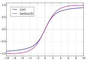
In the classical limit, the moments can be continuously aligned in the field and $J$ can assume all values ( $J\to \infty$ ). The Brillouin function is then simplified into the Langevin function, named after Paul Langevin:

$L(x)=\coth(x)-{\frac {1}{x}}$

For small values of $x$ , the Langevin function can be approximated by a truncation of its Taylor series:

L(x)={\tfrac {1}{3}}x-{\tfrac {1}{45}}x^{3}+{\tfrac {2}{945}}x^{5}-{\tfrac {1}{4725}}x^{7}+\dots

An alternative better behaved approximation can be derived from the Lambert's continued fraction expansion of $tanh(x)$ :

L(x)={\frac {x}{3+{\tfrac {x^{2}}{5+{\tfrac {x^{2}}{7+{\tfrac {x^{2}}{9+\ldots }}}}}}}}

For small enough $x$ , both approximations are numerically better than a direct evaluation of the actual analytical expression, since the latter suffers from Loss of significance.

The inverse Langevin function $L -1 (x)$ is defined on the open interval (−1, 1). For small values of $x$ , it can be approximated by a truncation of its Taylor series^[4]

L^{{-1}}(x)=3x+{\tfrac {9}{5}}x^{3}+{\tfrac {297}{175}}x^{5}+{\tfrac {1539}{875}}x^{7}+\dots

and by the Padé approximant

L^{{-1}}(x)=3x{\frac {35-12x^{2}}{35-33x^{2}}}+O(x^{7}).

Graphs of relative error for x ∈ [0, 1) for Cohen and Jedynak approximations

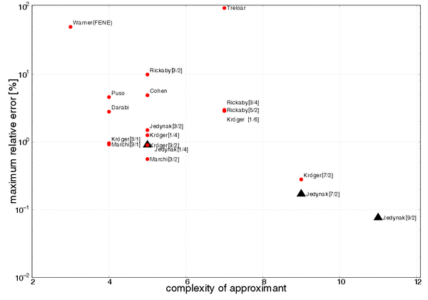
Since this function has no closed form, it is useful to have approximations valid for arbitrary values of $x$ . One popular approximation, valid on the whole range (−1, 1), has been published by A. Cohen:^[5]

L^{{-1}}(x)\approx x{\frac {3-x^{2}}{1-x^{2}}}.

This has a maximum relative error of 4.9% at the vicinity of $x = \pm0.8$ . Greater accuracy can be achieved by using the formula given by R. Jedynak:^[6]

L^{{-1}}(x)\approx x{\frac {3.0-2.6x+0.7x^{2}}{(1-x)(1+0.1x)}},

valid for $x \geq 0$ . The maximal relative error for this approximation is 1.5% at the vicinity of x = 0.85. Even greater accuracy can be achieved by using the formula given by M. Kröger:^[7]

L^{-1}(x)\approx {\frac {3x-x(6x^{2}+x^{4}-2x^{6})/5}{1-x^{2}}}

The maximal relative error for this approximation is less than 0.28%. More accurate approximation was reported by R. Petrosyan:^[8]

L^{-1}(x)\approx 3x+{\frac {x^{2}}{5}}\sin \left({\frac {7x}{2}}\right)+{\frac {x^{3}}{1-x}},

valid for $x \geq 0$ . The maximal relative error for the above formula is less than 0.18%.^[8]

New approximation given by R. Jedynak,^[9] is the best reported approximant at complexity 11:

$L^{-1}(x)\approx {\frac {x(3-1.00651x^{2}-0.962251x^{4}+1.47353x^{6}-0.48953x^{8})}{(1-x)(1+1.01524x)}},$

valid for $x \geq 0$ . Its maximum relative error is less than 0.076%.^[9]

Current state-of-the-art diagram of the approximants to the inverse Langevin function presents the figure below. It is valid for the rational/Padé approximants,^[7]^[9]

Current state-of-the-art diagram of the approximants to the inverse Langevin function,^[7]^[9]

High-temperature limit

When $x\ll 1$ i.e. when $\mu _{B}B/k_{B}T$ is small, the expression of the magnetization can be approximated by the Curie's law:

M=C\cdot {\frac {B}{T}}

where $C={\frac {Ng^{2}J(J+1)\mu _{B}^{2}}{3k_{B}}}$ is a constant. One can note that $g{\sqrt {J(J+1)}}$ is the effective number of Bohr magnetons.

High-field limit

When $x\to \infty$ , the Brillouin function goes to 1. The magnetization saturates with the magnetic moments completely aligned with the applied field:

M=Ng\mu _{B}J

References

1 2 3 C. Kittel, Introduction to Solid State Physics (8th ed.), pages 303-4 ISBN 978-0-471-41526-8
↑ Darby, M.I. (1967). "Tables of the Brillouin function and of the related function for the spontaneous magnetization". Br. J. Appl. Phys. 18 (10): 1415–1417. Bibcode:1967BJAP...18.1415D. doi:10.1088/0508-3443/18/10/307.
↑ Takacs, Jeno (2016). "Approximations for Brillouin and its reverse function". COMPEL. 35 (6): 2095.
↑ Johal, A. S.; Dunstan, D. J. (2007). "Energy functions for rubber from microscopic potentials". Journal of Applied Physics. 101 (8): 084917. Bibcode:2007JAP...101h4917J. doi:10.1063/1.2723870.
↑ Cohen, A. (1991). "A Padé approximant to the inverse Langevin function". Rheologica Acta. 30 (3): 270–273. doi:10.1007/BF00366640.
↑ Jedynak, R. (2015). "Approximation of the inverse Langevin function revisited". Rheologica Acta. 54 (1): 29–39. doi:10.1007/s00397-014-0802-2.
1 2 3 Kröger, M. (2015). "Simple, admissible, and accurate approximants of the inverse Langevin and Brillouin functions, relevant for strong polymer deformations and flows". J Non-Newton Fluid Mech. 223: 77–87. doi:10.1016/j.jnnfm.2015.05.007.
1 2 Petrosyan, R. (2016). "Improved approximations for some polymer extension models". Rheologica Acta. arXiv:1606.02519. doi:10.1007/s00397-016-0977-9.
1 2 3 4 Jedynak, R. (2017). "New facts concerning the approximation of the inverse Langevin function". Journal of Non-Newtonian Fluid Mechanics. 249: 8–25. doi:10.1016/j.jnnfm.2017.09.003.

This article is issued from Wikipedia. The text is licensed under Creative Commons - Attribution - Sharealike. Additional terms may apply for the media files.

[Kittel-1] 1 2 3 C. Kittel, Introduction to Solid State Physics (8th ed.), pages 303-4 ISBN 978-0-471-41526-8

[2] Darby, M.I. (1967). "Tables of the Brillouin function and of the related function for the spontaneous magnetization". Br. J. Appl. Phys. 18 (10): 1415–1417. Bibcode:1967BJAP...18.1415D. doi:10.1088/0508-3443/18/10/307.

[3] Takacs, Jeno (2016). "Approximations for Brillouin and its reverse function". COMPEL. 35 (6): 2095.

[Johal-4] Johal, A. S.; Dunstan, D. J. (2007). "Energy functions for rubber from microscopic potentials". Journal of Applied Physics. 101 (8): 084917. Bibcode:2007JAP...101h4917J. doi:10.1063/1.2723870.

[Cohen-5] Cohen, A. (1991). "A Padé approximant to the inverse Langevin function". Rheologica Acta. 30 (3): 270–273. doi:10.1007/BF00366640.

[Jedynak-6] Jedynak, R. (2015). "Approximation of the inverse Langevin function revisited". Rheologica Acta. 54 (1): 29–39. doi:10.1007/s00397-014-0802-2.

[M._Kröger-7] 1 2 3 Kröger, M. (2015). "Simple, admissible, and accurate approximants of the inverse Langevin and Brillouin functions, relevant for strong polymer deformations and flows". J Non-Newton Fluid Mech. 223: 77–87. doi:10.1016/j.jnnfm.2015.05.007.

[Petrosyan-8] 1 2 Petrosyan, R. (2016). "Improved approximations for some polymer extension models". Rheologica Acta. arXiv:1606.02519. doi:10.1007/s00397-016-0977-9.

[Jedynak1-9] 1 2 3 4 Jedynak, R. (2017). "New facts concerning the approximation of the inverse Langevin function". Journal of Non-Newtonian Fluid Mechanics. 249: 8–25. doi:10.1016/j.jnnfm.2017.09.003.