Backpropagation

Backpropagation is a method used in artificial neural networks to calculate a gradient that is needed in the calculation of the weights to be used in the network.^[1] It is commonly used to train deep neural networks,^[2] a term referring to neural networks with more than one hidden layer.^[3]

Backpropagation is a special case of a more general technique called automatic differentiation. In the context of learning, backpropagation is commonly used by the gradient descent optimization algorithm to adjust the weight of neurons by calculating the gradient of the loss function. This technique is also sometimes called backward propagation of errors, because the error is calculated at the output and distributed back through the network layers.

Backpropagation requires the derivative of the loss function with respect to the network output to be known, which typically (but not necessarily) means that a desired target value is known. For this reason it is considered to be a supervised learning method, although it is used in some unsupervised networks such as autoencoders. Backpropagation is also a generalization of the delta rule to multi-layered feedforward networks, made possible by using the chain rule to iteratively compute gradients for each layer. It is closely related to the Gauss–Newton algorithm, and is part of continuing research in neural backpropagation. Backpropagation can be used with any gradient-based optimizer, such as L-BFGS or truncated Newton.

History

Backpropagation was derived by multiple researchers in the early 60's^[4] and implemented to run on computers much as it is today as early as 1970 by Seppo Linnainmaa^[5]^[6]^[7] Examples of 1960s researchers include Arthur E. Bryson and Yu-Chi Ho in 1969.^[8]^[9] Paul Werbos was first in the US to propose that it could be used for neural nets after analyzing it in depth in his 1974 PhD Thesis.^[10] In 1986 through the work of David E. Rumelhart, Geoffrey E. Hinton, Ronald J. Williams^[11], and James McClelland^[12], backpropagation gained recognition.

Motivation

The goal of any supervised learning algorithm is to find a function that best maps a set of inputs to their correct output. An example would be a classification task, where the input is an image of an animal, and the correct output is the type of animal (e.g.: dog, cat, giraffe, lion, zebra, etc.).

The motivation for backpropagation is to train a multi-layered neural network such that it can learn the appropriate internal representations to allow it to learn any arbitrary mapping of input to output.^[13]

Loss function

Sometimes referred to as the cost function or error function (not to be confused with the Gauss error function), the loss function is a function that maps values of one or more variables onto a real number intuitively representing some "cost" associated with those values. For backpropagation, the loss function calculates the difference between the network output and its expected output, after a case propagates through the network.

Assumptions

Two assumptions must be made about the form of the error function.^[14] The first is that it can be written as an average ${\textstyle E={\frac {1}{n}}\sum _{x}E_{x}}$ over error functions ${\textstyle E_{x}}$ , for ${\textstyle n}$ individual training examples, ${\textstyle x}$ . The reason for this assumption is that the backpropagation algorithm calculates the gradient of the error function for a single training example, which needs to be generalized to the overall error function. The second assumption is that it can be written as a function of the outputs from the neural network.

Example loss function

Let $y,y'$ be vectors in $\mathbb {R} ^{n}$ .

Select an error function $E(y,y')$ measuring the difference between two outputs. The standard choice is the square of the Euclidean distance between the vectors $y$ and $y'$ :

E(y,y')={\tfrac {1}{2}}\lVert y-y'\rVert ^{2}

and therefore, the partial derivative with respect to the outputs:

{\frac {\partial E}{\partial y'}}=y'-y

The error function over ${\textstyle n}$ training examples can simply be written as an average of losses over individual examples:

E={\frac {1}{2n}}\sum _{x}\lVert (y(x)-y'(x))\rVert ^{2}

Optimization

The optimization algorithm repeats a two phase cycle, propagation and weight update. When an input vector is presented to the network, it is propagated forward through the network, layer by layer, until it reaches the output layer. The output of the network is then compared to the desired output, using a loss function. The resulting error value is calculated for each of the neurons in the output layer. The error values are then propagated from the output back through the network, until each neuron has an associated error value that reflects its contribution to the original output.

Backpropagation uses these error values to calculate the gradient of the loss function. In the second phase, this gradient is fed to the optimization method, which in turn uses it to update the weights, in an attempt to minimize the loss function.

Algorithm

Let $N$ be a neural network with $e$ connections, $m$ inputs, and $n$ outputs.

Below, $x_{1},x_{2},\dots$ will denote vectors in $\mathbb {R} ^{m}$ , $y_{1},y_{2},\dots$ vectors in $\mathbb {R} ^{n}$ , and $w_{0},w_{1},w_{2},\ldots$ vectors in $\mathbb {R} ^{e}$ . These are called inputs, outputs and weights respectively.

The neural network corresponds to a function $y=f_{N}(w,x)$ which, given a weight $w$ , maps an input $x$ to an output $y$ .

The optimization takes as input a sequence of training examples $(x_{1},y_{1}),\dots ,(x_{p},y_{p})$ and produces a sequence of weights $w_{0},w_{1},\dots ,w_{p}$ starting from some initial weight $w_{0}$ , usually chosen at random.

These weights are computed in turn: first compute $w_{i}$ using only $(x_{i},y_{i},w_{i-1})$ for $i=1,\dots ,p$ . The output of the algorithm is then $w_p$ , giving us a new function $x\mapsto f_{N}(w_{p},x)$ . The computation is the same in each step, hence only the case $i=1$ is described.

Calculating $w_{1}$ from $(x_{1},y_{1},w_{0})$ is done by considering a variable weight $w$ and applying gradient descent to the function $w\mapsto E(f_{N}(w,x_{1}),y_{1})$ to find a local minimum, starting at $w=w_{0}$ .

This makes $w_{1}$ the minimizing weight found by gradient descent.

Algorithm in code

To implement the algorithm above, explicit formulas are required for the gradient of the function $w\mapsto E(f_{N}(w,x),y)$ where the function is $E(y,y')=|y-y'|^{2}$ .

The learning algorithm can be divided into two phases: propagation and weight update.

Phase 1: propagation

Each propagation involves the following steps:

Propagation forward through the network to generate the output value(s)
Calculation of the cost (error term)
Propagation of the output activations back through the network using the training pattern target in order to generate the deltas (the difference between the targeted and actual output values) of all output and hidden neurons.

Phase 2: weight update

For each weight, the following steps must be followed:

The weight's output delta and input activation are multiplied to find the gradient of the weight.
A ratio (percentage) of the weight's gradient is subtracted from the weight.

This ratio (percentage) influences the speed and quality of learning; it is called the learning rate. The greater the ratio, the faster the neuron trains, but the lower the ratio, the more accurate the training is. The sign of the gradient of a weight indicates whether the error varies directly with, or inversely to, the weight. Therefore, the weight must be updated in the opposite direction, "descending" the gradient.

Learning is repeated (on new batches) until the network performs adequately.

Pseudocode

The following is pseudocode for a stochastic gradient descent algorithm for training a three-layer network (only one hidden layer):

  initialize network weights (often small random values)
  do
     forEach training example named ex
        prediction = neural-net-output(network, ex)  // forward pass
        actual = teacher-output(ex)
        compute error (prediction - actual) at the output units
        compute  $\Delta w_h$ 
 for all weights from hidden layer to output layer  // backward pass
        compute  $\Delta w_i$ 
 for all weights from input layer to hidden layer   // backward pass continued
        update network weights // input layer not modified by error estimate
  until all examples classified correctly or another stopping criterion satisfied
  return the network

The lines labeled "backward pass" can be implemented using the backpropagation algorithm, which calculates the gradient of the error of the network regarding the network's modifiable weights.^[15]

Intuition

Learning as an optimization problem

To understand the mathematical derivation of the backpropagation algorithm, it helps to first develop some intuitions about the relationship between the actual output of a neuron and the correct output for a particular training case. Consider a simple neural network with two input units, one output unit and no hidden units. Each neuron uses a linear output^{[note 1]} that is the weighted sum of its input.

A simple neural network with two input units and one output unit

Initially, before training, the weights will be set randomly. Then the neuron learns from training examples, which in this case consists of a set of tuples $(x_{1},x_{2},t)$ where $x_{1}$ and $x_{2}$ are the inputs to the network and $t$ is the correct output (the output the network should eventually produce given those inputs). The initial network, given $x_{1}$ and $x_{2}$ , will compute an output $y$ that likely differs from $t$ (given random weights). A common method for measuring the discrepancy between the expected output $t$ and the actual output $y$ is the squared error measure:

E=(t-y)^{2},

where $E$ is the discrepancy or error.

As an example, consider the network on a single training case: $(1, 1, 0)$ , thus the input $x_{1}$ and $x_{2}$ are 1 and 1 respectively and the correct output, $t$ is 0. Now if the actual output $y$ is plotted on the horizontal axis against the error $E$ on the vertical axis, the result is a parabola. The minimum of the parabola corresponds to the output $y$ which minimizes the error $E$ . For a single training case, the minimum also touches the horizontal axis, which means the error will be zero and the network can produce an output $y$ that exactly matches the expected output $t$ . Therefore, the problem of mapping inputs to outputs can be reduced to an optimization problem of finding a function that will produce the minimal error.

Error surface of a linear neuron for a single training case.

However, the output of a neuron depends on the weighted sum of all its inputs:

y=x_{1}w_{1}+x_{2}w_{2},

where $w_{1}$ and $w_{2}$ are the weights on the connection from the input units to the output unit. Therefore, the error also depends on the incoming weights to the neuron, which is ultimately what needs to be changed in the network to enable learning. If each weight is plotted on a separate horizontal axis and the error on the vertical axis, the result is a parabolic bowl. For a neuron with $k$ weights, the same plot would require an elliptic paraboloid of $k+1$ dimensions.

Error surface of a linear neuron with two input weights

One commonly used algorithm to find the set of weights that minimizes the error is gradient descent. Backpropagation is then used to calculate the steepest descent direction.

Derivation for a single-layered network

The gradient descent method involves calculating the derivative of the squared error function with respect to the weights of the network. This is normally done using backpropagation. Assuming one output neuron,^{[note 2]} the squared error function is:

E={\tfrac {1}{2}}(t-y)^{2},

where

E

is the squared error,

t

is the target output for a training sample, and

y

is the actual output of the output neuron.

The factor of $\textstyle {\frac {1}{2}}$ is included to cancel the exponent when differentiating. Later, the expression will be multiplied with an arbitrary learning rate, so that it doesn't matter if a constant coefficient is introduced now.

For each neuron $j$ , its output $o_j$ is defined as

o_{j}=\varphi ({\text{net}}_{j})=\varphi \left(\sum _{k=1}^{n}w_{kj}o_{k}\right).

The input ${\text{net}}_{j}$ to a neuron is the weighted sum of outputs $o_k$ of previous neurons. If the neuron is in the first layer after the input layer, the $o_k$ of the input layer are simply the inputs $x_{k}$ to the network. The number of input units to the neuron is $n$ . The variable $w_{kj}$ denotes the weight between neurons $k$ and $j$ .

The activation function $\varphi$ is non-linear and differentiable. A commonly used activation function is the logistic function:

\varphi (z)={\frac {1}{1+e^{-z}}}

which has a convenient derivative of:

{\frac {d\varphi }{dz}}(z)=\varphi (z)(1-\varphi (z))

Finding the derivative of the error

Calculating the partial derivative of the error with respect to a weight $w_{ij}$ is done using the chain rule twice:

{\frac {\partial E}{\partial w_{ij}}}={\frac {\partial E}{\partial o_{j}}}{\frac {\partial o_{j}}{\partial {\text{net}}_{j}}}{\frac {\partial {\text{net}}_{j}}{\partial w_{ij}}}

In the last factor of the right-hand side of the above, only one term in the sum ${\text{net}}_{j}$ depends on $w_{ij}$ , so that

{\frac {\partial {\text{net}}_{j}}{\partial w_{ij}}}={\frac {\partial }{\partial w_{ij}}}\left(\sum _{k=1}^{n}w_{kj}o_{k}\right)={\frac {\partial }{\partial w_{ij}}}w_{ij}o_{i}=o_{i}.

If the neuron is in the first layer after the input layer, $o_i$ is just $x_{i}$ .

The derivative of the output of neuron $j$ with respect to its input is simply the partial derivative of the activation function (assuming here that the logistic function is used):

{\frac {\partial o_{j}}{\partial {\text{net}}_{j}}}={\frac {\partial }{\partial {\text{net}}_{j}}}\varphi ({\text{net}}_{j})=\varphi ({\text{net}}_{j})(1-\varphi ({\text{net}}_{j}))

This is the reason why backpropagation requires the activation function to be differentiable. (Nevertheless, the non-differentiable ReLU activation function has become quite popular recently, e.g. in AlexNet)

The first factor is straightforward to evaluate if the neuron is in the output layer, because then $o_j = y$ and

\frac{\partial E}{\partial o_j} = \frac{\partial E}{\partial y} = \frac{\partial}{\partial y} \frac{1}{2}(t - y)^2 = y - t

However, if $j$ is in an arbitrary inner layer of the network, finding the derivative $E$ with respect to $o_j$ is less obvious.

Considering $E$ as a function of the inputs of all neurons $L = {u, v, \dots, w}$ receiving input from neuron $j$ ,

{\frac {\partial E(o_{j})}{\partial o_{j}}}={\frac {\partial E(\mathrm {net} _{u},{\text{net}}_{v},\dots ,\mathrm {net} _{w})}{\partial o_{j}}}

and taking the total derivative with respect to $o_j$ , a recursive expression for the derivative is obtained:

{\frac {\partial E}{\partial o_{j}}}=\sum _{\ell \in L}\left({\frac {\partial E}{\partial {\text{net}}_{\ell }}}{\frac {\partial {\text{net}}_{\ell }}{\partial o_{j}}}\right)=\sum _{\ell \in L}\left({\frac {\partial E}{\partial o_{\ell }}}{\frac {\partial o_{\ell }}{\partial {\text{net}}_{\ell }}}w_{j\ell }\right)

Therefore, the derivative with respect to $o_j$ can be calculated if all the derivatives with respect to the outputs $o_{\ell }$ of the next layer – the one closer to the output neuron – are known.

Putting it all together:

{\frac {\partial E}{\partial w_{ij}}}=\delta _{j}o_{i}

with

\delta _{j}={\frac {\partial E}{\partial o_{j}}}{\frac {\partial o_{j}}{\partial {\text{net}}_{j}}}={\begin{cases}(o_{j}-t_{j})o_{j}(1-o_{j})&{\text{if }}j{\text{ is an output neuron,}}\\(\sum _{\ell \in L}w_{j\ell }\delta _{\ell })o_{j}(1-o_{j})&{\text{if }}j{\text{ is an inner neuron.}}\end{cases}}

To update the weight $w_{ij}$ using gradient descent, one must choose a learning rate, $\eta >0$ . The change in weight needs to reflect the impact on $E$ of an increase or decrease in $w_{ij}$ . If ${\frac {\partial E}{\partial w_{ij}}}>0$ , an increase in $w_{ij}$ increases $E$ ; conversely, if ${\frac {\partial E}{\partial w_{ij}}}<0$ , an increase in $w_{ij}$ decreases $E$ . The new $\Delta w_{ij}$ is added to the old weight, and the product of the learning rate and the gradient, multiplied by $-1$ guarantees that $w_{ij}$ changes in a way that always decreases $E$ . In other words, in the equation immediately below, $-\eta {\frac {\partial E}{\partial w_{ij}}}$ always changes $w_{ij}$ in such a way that $E$ is decreased:

\Delta w_{ij}=-\eta {\frac {\partial E}{\partial w_{ij}}}=-\eta \delta _{j}o_{i}

Extension

The choice of learning rate ${\textstyle \eta }$ is important, since a high value can cause too strong a change, causing the minimum to be missed, while a too low learning rate slows the training unnecessarily.

Optimizations such as Quickprop are primarily aimed at speeding up error minimization; other improvements mainly try to increase reliability.

Adaptive learning rate

In order to avoid oscillation inside the network such as alternating connection weights, and to improve the rate of convergence, refinements of this algorithm use an adaptive learning rate.^[16]

Inertia

By using a variable inertia term (Momentum) ${\textstyle \alpha }$ the gradient and the last change can be weighted such that the weight adjustment additionally depends on the previous change. If the Momentum ${\textstyle \alpha }$ is equal to 0, the change depends solely on the gradient, while a value of 1 will only depend on the last change.

Similar to a ball rolling down a mountain, whose current speed is determined not only by the current slope of the mountain but also by its own inertia, inertia can be added:

\Delta w_{ij}(t+1)=(1-\alpha )\eta \delta _{j}o_{i}+\alpha \,\Delta w_{ij}(t)

where:

{\textstyle \Delta w_{ij}(t+1)}

is the change in weight

{\textstyle w_{ij}(t+1)}

in the connection of neuron

{\textstyle i}

to neuron

{\textstyle j}

at time

{\textstyle (t+1),}

{\textstyle \eta }

a learning rate (

{\textstyle \eta <0),}

{\textstyle \delta _{j}}

the error signal of neuron

{\textstyle j}

and

{\textstyle o_{i}}

the output of neuron

{\textstyle i}

, which is also an input of the current neuron (neuron

{\textstyle j}

),

{\textstyle \alpha }

the influence of the inertial term

{\textstyle \Delta w_{ij}(t)}

(in

{\textstyle [0,1]}

). This corresponds to the weight change at the previous point in time.

Inertia depends on the current weight change ${\textstyle (t+1)}$ both from the current gradient of the error function (slope of the mountain, 1st summand), as well as from the weight change from the previous point in time (inertia, 2nd summand).

With inertia, the problems of getting stuck (in steep ravines and flat plateaus) are avoided. Since, for example, the gradient of the error function becomes very small in flat plateaus, inertia would immediately lead to a "deceleration" of the gradient descent. This deceleration is delayed by the addition of the inertia term so that a flat plateau can be escaped more quickly.

Modes of learning

Two modes of learning are available: stochastic and batch. In stochastic learning, each input creates a weight adjustment. In batch learning weights are adjusted based on a batch of inputs, accumulating errors over the batch. Stochastic learning introduces "noise" into the gradient descent process, using the local gradient calculated from one data point; this reduces the chance of the network getting stuck in local minima. However, batch learning typically yields a faster, more stable descent to a local minimum, since each update is performed in the direction of the average error of the batch. A common compromise choice is to use "mini-batches", meaning small batches and with samples in each batch selected stochastically from the entire data set.

Limitations

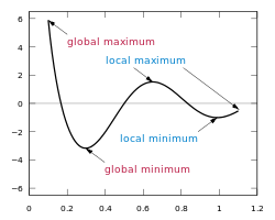
Gradient descent can find the local minimum instead of the global minimum

Gradient descent with backpropagation is not guaranteed to find the global minimum of the error function, but only a local minimum; also, it has trouble crossing plateaus in the error function landscape. This issue, caused by the non-convexity of error functions in neural networks, was long thought to be a major drawback, but Yann LeCun et al. argue that in many practical problems, it is not.^[17]
Backpropagation learning does not require normalization of input vectors; however, normalization could improve performance.^[18]

History

According to various sources,^[19]^[20]^[21]^[22]^[23] the basics of continuous backpropagation were derived in the context of control theory by Henry J. Kelley^[24] in 1960 and by Arthur E. Bryson in 1961.^[25] They used principles of dynamic programming. In 1962, Stuart Dreyfus published a simpler derivation based only on the chain rule.^[26] Bryson and Ho described it as a multi-stage dynamic system optimization method in 1969.^[27]^[28]

In 1970 Linnainmaa published the general method for automatic differentiation (AD) of discrete connected networks of nested differentiable functions.^[6]^[7] This corresponds to backpropagation, which is efficient even for sparse networks.^[22]^[23]^[29]^[30]

In 1973 Dreyfus used backpropagation to adapt parameters of controllers in proportion to error gradients.^[31] In 1974 Werbos mentioned the possibility of applying this principle to artificial neural networks,^[32] and in 1982 he applied Linnainmaa's AD method to neural networks in the way that is used today.^[23]^[33]

In 1986 Rumelhart, Hinton and Williams showed experimentally that this method can generate useful internal representations of incoming data in hidden layers of neural networks.^[13]^[34] In 1993, Wan was the first^[22] to win an international pattern recognition contest through backpropagation.^[35]

During the 2000s it fell out of favour, but returned in the 2010s, benefitting from cheap, powerful GPU-based computing systems. This has been especially so in language structure learning research, where the connectionist models using this algorithm have been able to explain a variety of phenomena related to first ^[36] and second language learning. ^[37]

Notes

↑ One may notice that multi-layer neural networks use non-linear activation functions, so an example with linear neurons seems obscure. However, even though the error surface of multi-layer networks are much more complicated, locally they can be approximated by a paraboloid. Therefore, linear neurons are used for simplicity and easier understanding.
↑ There can be multiple output neurons, in which case the error is the squared norm of the difference vector.

References

↑ Deep Learning; Ian Goodfellow, Yoshua Bengio, Aaaron Courville; MIT Press; 2016, p 196
↑ Nielsen, Michael A. (2015). "Chapter 6". Neural Networks and Deep Learning.
↑ "Deep Networks: Overview - Ufldl". ufldl.stanford.edu. Retrieved 2017-08-04.
↑ Schmidhuber, Jürgen (2015-01-01). "Deep learning in neural networks: An overview". Neural Networks. 61: 85–117. arXiv:1404.7828. doi:10.1016/j.neunet.2014.09.003. ISSN 0893-6080. PMID 25462637.
↑ Griewank, Andreas (2012). Who Invented the Reverse Mode of Differentiation?. Optimization Stories, Documenta Matematica, Extra Volume ISMP (2012), 389-400.
1 2 Seppo Linnainmaa (1970). The representation of the cumulative rounding error of an algorithm as a Taylor expansion of the local rounding errors. Master's Thesis (in Finnish), Univ. Helsinki, 6–7.
1 2 Linnainmaa, Seppo (1976). "Taylor expansion of the accumulated rounding error". BIT Numerical Mathematics. 16 (2): 146–160. doi:10.1007/bf01931367.
↑ Stuart Russell and Peter Norvig. Artificial Intelligence A Modern Approach. p. 578. The most popular method for learning in multilayer networks is called Back-propagation. It was first invented in 1969 by Bryson and Ho, but was more or less ignored until the mid-1980s.
↑ Bryson, Arthur Earl; Ho, Yu-Chi (1969). Applied optimal control: optimization, estimation, and control. Blaisdell Publishing Company or Xerox College Publishing. p. 481.
↑ Werbos, P.. Beyond Regression: New Tools for Prediction and Analysis in the Behavioral Sciences. PhD thesis, Harvard University, 1974
↑ Rumelhart, David E.; Hinton, Geoffrey E.; Williams, Ronald J. (1986-10-09). "Learning representations by back-propagating errors". Nature. 323 (6088): 533–536. Bibcode:1986Natur.323..533R. doi:10.1038/323533a0. ISSN 1476-4687.
↑ Rumelhart, David E; Mcclelland, James L (1986-01-01). Parallel distributed processing: explorations in the microstructure of cognition. Volume 1. Foundations.
1 2 Rumelhart, David E.; Hinton, Geoffrey E.; Williams, Ronald J. (8 October 1986). "Learning representations by back-propagating errors". Nature. 323 (6088): 533–536. Bibcode:1986Natur.323..533R. doi:10.1038/323533a0.
↑ A., Nielsen, Michael (2015-01-01). "Neural Networks and Deep Learning".
↑ Paul J. Werbos (1994). The Roots of Backpropagation. From Ordered Derivatives to Neural Networks and Political Forecasting. New York, NY: John Wiley & Sons, Inc.
↑ Li, Y.; Fu, Y.; Li, H.; Zhang, S. W. (2009-06-01). The Improved Training Algorithm of Back Propagation Neural Network with Self-adaptive Learning Rate. 2009 International Conference on Computational Intelligence and Natural Computing. 1. pp. 73–76. doi:10.1109/CINC.2009.111. ISBN 978-0-7695-3645-3.
↑ LeCun, Yann; Bengio, Yoshua; Hinton, Geoffrey (2015). "Deep learning". Nature. 521 (7553): 436–444. Bibcode:2015Natur.521..436L. doi:10.1038/nature14539. PMID 26017442.
↑ Buckland, Matt; Collins, Mark. AI Techniques for Game Programming. ISBN 978-1-931841-08-5.
↑ DREYFUS, STUART E. (1990). "Artificial neural networks, back propagation, and the Kelley-Bryson gradient procedure". Journal of Guidance, Control, and Dynamics. 13 (5): 926–928. Bibcode:1990JGCD...13..926D. doi:10.2514/3.25422. ISSN 0731-5090.
↑ Stuart Dreyfus (1990). Artificial Neural Networks, Back Propagation and the Kelley-Bryson Gradient Procedure. J. Guidance, Control and Dynamics, 1990.
↑ Mizutani, Eiji; Dreyfus, Stuart; Nishio, Kenichi (July 2000). "On derivation of MLP backpropagation from the Kelley-Bryson optimal-control gradient formula and its application" (PDF). Proceedings of the IEEE International Joint Conference on Neural Networks.
1 2 3 Schmidhuber, Jürgen (2015). "Deep learning in neural networks: An overview". Neural Networks. 61: 85–117. arXiv:1404.7828. doi:10.1016/j.neunet.2014.09.003. PMID 25462637.
1 2 3 Schmidhuber, Jürgen (2015). "Deep Learning". Scholarpedia. 10 (11): 32832. Bibcode:2015SchpJ..1032832S. doi:10.4249/scholarpedia.32832.
↑ Kelley, Henry J. (1960). "Gradient theory of optimal flight paths". ARS Journal. 30 (10): 947–954. Bibcode:1960ARSJ...30.1127B. doi:10.2514/8.5282.
↑ Arthur E. Bryson (1961, April). A gradient method for optimizing multi-stage allocation processes. In Proceedings of the Harvard Univ. Symposium on digital computers and their applications.
↑ Dreyfus, Stuart (1962). "The numerical solution of variational problems". Journal of Mathematical Analysis and Applications. 5 (1): 30–45. doi:10.1016/0022-247x(62)90004-5.
↑ Stuart Russell; Peter Norvig. Artificial Intelligence A Modern Approach. p. 578. The most popular method for learning in multilayer networks is called Back-propagation.
↑ Bryson, A. E.; Yu-Chi, Ho (1 January 1975). Applied Optimal Control: Optimization, Estimation and Control. CRC Press. ISBN 978-0-89116-228-5.
↑ "Who Invented the Reverse Mode of Differentiation? - Semantic Scholar". www.semanticscholar.org. 2012. Retrieved 2017-08-04.
↑ Griewank, Andreas; Walther, Andrea (2008). Evaluating Derivatives: Principles and Techniques of Algorithmic Differentiation, Second Edition. SIAM. ISBN 978-0-89871-776-1.
↑ Dreyfus, Stuart (1973). "The computational solution of optimal control problems with time lag". IEEE Transactions on Automatic Control. 18 (4): 383–385. doi:10.1109/tac.1973.1100330.
↑ Werbos, Paul John (1975). Beyond Regression: New Tools for Prediction and Analysis in the Behavioral Sciences. Harvard University.
↑ Werbos, Paul (1982). "Applications of advances in nonlinear sensitivity analysis". System modeling and optimization (PDF). Springer. pp. 762–770.
↑ Alpaydin, Ethem (2010). Introduction to Machine Learning. MIT Press. ISBN 978-0-262-01243-0.
↑ Wan, Eric A. (1993). "Time series prediction by using a connectionist network with internal delay lines" (PDF). SANTA FE INSTITUTE STUDIES IN THE SCIENCES OF COMPLEXITY-PROCEEDINGS. p. 195.
↑ Chang, Franklin; Dell, Gary S.; Bock, Kathryn (2006). "Becoming syntactic". Psychological Review. 113 (2): 234–272. doi:10.1037/0033-295x.113.2.234. ISSN 1939-1471. PMID 16637761.
↑ Janciauskas, Marius; Chang, Franklin (2017-07-26). "Input and Age-Dependent Variation in Second Language Learning: A Connectionist Account". Cognitive Science. 42: 519–554. doi:10.1111/cogs.12519. ISSN 0364-0213. PMC 6001481. PMID 28744901.

External links

This article is issued from Wikipedia. The text is licensed under Creative Commons - Attribution - Sharealike. Additional terms may apply for the media files.

[16] One may notice that multi-layer neural networks use non-linear activation functions, so an example with linear neurons seems obscure. However, even though the error surface of multi-layer networks are much more complicated, locally they can be approximated by a paraboloid. Therefore, linear neurons are used for simplicity and easier understanding.

[17] There can be multiple output neurons, in which case the error is the squared norm of the difference vector.

[1] Deep Learning; Ian Goodfellow, Yoshua Bengio, Aaaron Courville; MIT Press; 2016, p 196

[2] Nielsen, Michael A. (2015). "Chapter 6". Neural Networks and Deep Learning.

[3] "Deep Networks: Overview - Ufldl". ufldl.stanford.edu. Retrieved 2017-08-04.

[4] Schmidhuber, Jürgen (2015-01-01). "Deep learning in neural networks: An overview". Neural Networks. 61: 85–117. arXiv:1404.7828. doi:10.1016/j.neunet.2014.09.003. ISSN 0893-6080. PMID 25462637.

[grie2012-5] Griewank, Andreas (2012). Who Invented the Reverse Mode of Differentiation?. Optimization Stories, Documenta Matematica, Extra Volume ISMP (2012), 389-400.

[lin1970-6] 1 2 Seppo Linnainmaa (1970). The representation of the cumulative rounding error of an algorithm as a Taylor expansion of the local rounding errors. Master's Thesis (in Finnish), Univ. Helsinki, 6–7.

[lin1976-7] 1 2 Linnainmaa, Seppo (1976). "Taylor expansion of the accumulated rounding error". BIT Numerical Mathematics. 16 (2): 146–160. doi:10.1007/bf01931367.

[8] Stuart Russell and Peter Norvig. Artificial Intelligence A Modern Approach. p. 578. The most popular method for learning in multilayer networks is called Back-propagation. It was first invented in 1969 by Bryson and Ho, but was more or less ignored until the mid-1980s.

[9] Bryson, Arthur Earl; Ho, Yu-Chi (1969). Applied optimal control: optimization, estimation, and control. Blaisdell Publishing Company or Xerox College Publishing. p. 481.

[10] Werbos, P.. Beyond Regression: New Tools for Prediction and Analysis in the Behavioral Sciences. PhD thesis, Harvard University, 1974

[11] Rumelhart, David E.; Hinton, Geoffrey E.; Williams, Ronald J. (1986-10-09). "Learning representations by back-propagating errors". Nature. 323 (6088): 533–536. Bibcode:1986Natur.323..533R. doi:10.1038/323533a0. ISSN 1476-4687.

[12] Rumelhart, David E; Mcclelland, James L (1986-01-01). Parallel distributed processing: explorations in the microstructure of cognition. Volume 1. Foundations.

[Rumelhart1986-13] 1 2 Rumelhart, David E.; Hinton, Geoffrey E.; Williams, Ronald J. (8 October 1986). "Learning representations by back-propagating errors". Nature. 323 (6088): 533–536. Bibcode:1986Natur.323..533R. doi:10.1038/323533a0.

[:0-14] A., Nielsen, Michael (2015-01-01). "Neural Networks and Deep Learning".

[15] Paul J. Werbos (1994). The Roots of Backpropagation. From Ordered Derivatives to Neural Networks and Political Forecasting. New York, NY: John Wiley & Sons, Inc.

[18] Li, Y.; Fu, Y.; Li, H.; Zhang, S. W. (2009-06-01). The Improved Training Algorithm of Back Propagation Neural Network with Self-adaptive Learning Rate. 2009 International Conference on Computational Intelligence and Natural Computing. 1. pp. 73–76. doi:10.1109/CINC.2009.111. ISBN 978-0-7695-3645-3.

[19] LeCun, Yann; Bengio, Yoshua; Hinton, Geoffrey (2015). "Deep learning". Nature. 521 (7553): 436–444. Bibcode:2015Natur.521..436L. doi:10.1038/nature14539. PMID 26017442.

[20] Buckland, Matt; Collins, Mark. AI Techniques for Game Programming. ISBN 978-1-931841-08-5.

[21] DREYFUS, STUART E. (1990). "Artificial neural networks, back propagation, and the Kelley-Bryson gradient procedure". Journal of Guidance, Control, and Dynamics. 13 (5): 926–928. Bibcode:1990JGCD...13..926D. doi:10.2514/3.25422. ISSN 0731-5090.

[dreyfus1990-22] Stuart Dreyfus (1990). Artificial Neural Networks, Back Propagation and the Kelley-Bryson Gradient Procedure. J. Guidance, Control and Dynamics, 1990.

[23] Mizutani, Eiji; Dreyfus, Stuart; Nishio, Kenichi (July 2000). "On derivation of MLP backpropagation from the Kelley-Bryson optimal-control gradient formula and its application" (PDF). Proceedings of the IEEE International Joint Conference on Neural Networks.

[schmidhuber2015-24] 1 2 3 Schmidhuber, Jürgen (2015). "Deep learning in neural networks: An overview". Neural Networks. 61: 85–117. arXiv:1404.7828. doi:10.1016/j.neunet.2014.09.003. PMID 25462637.

[scholarpedia2015-25] 1 2 3 Schmidhuber, Jürgen (2015). "Deep Learning". Scholarpedia. 10 (11): 32832. Bibcode:2015SchpJ..1032832S. doi:10.4249/scholarpedia.32832.

[kelley1960-26] Kelley, Henry J. (1960). "Gradient theory of optimal flight paths". ARS Journal. 30 (10): 947–954. Bibcode:1960ARSJ...30.1127B. doi:10.2514/8.5282.

[bryson1961-27] Arthur E. Bryson (1961, April). A gradient method for optimizing multi-stage allocation processes. In Proceedings of the Harvard Univ. Symposium on digital computers and their applications.

[28] Dreyfus, Stuart (1962). "The numerical solution of variational problems". Journal of Mathematical Analysis and Applications. 5 (1): 30–45. doi:10.1016/0022-247x(62)90004-5.

[29] Stuart Russell; Peter Norvig. Artificial Intelligence A Modern Approach. p. 578. The most popular method for learning in multilayer networks is called Back-propagation.

[30] Bryson, A. E.; Yu-Chi, Ho (1 January 1975). Applied Optimal Control: Optimization, Estimation and Control. CRC Press. ISBN 978-0-89116-228-5.

[31] "Who Invented the Reverse Mode of Differentiation? - Semantic Scholar". www.semanticscholar.org. 2012. Retrieved 2017-08-04.

[grie2008-32] Griewank, Andreas; Walther, Andrea (2008). Evaluating Derivatives: Principles and Techniques of Algorithmic Differentiation, Second Edition. SIAM. ISBN 978-0-89871-776-1.

[dreyfus1973-33] Dreyfus, Stuart (1973). "The computational solution of optimal control problems with time lag". IEEE Transactions on Automatic Control. 18 (4): 383–385. doi:10.1109/tac.1973.1100330.

[werbos1974-34] Werbos, Paul John (1975). Beyond Regression: New Tools for Prediction and Analysis in the Behavioral Sciences. Harvard University.

[werbos1982-35] Werbos, Paul (1982). "Applications of advances in nonlinear sensitivity analysis". System modeling and optimization (PDF). Springer. pp. 762–770.

[36] Alpaydin, Ethem (2010). Introduction to Machine Learning. MIT Press. ISBN 978-0-262-01243-0.

[37] Wan, Eric A. (1993). "Time series prediction by using a connectionist network with internal delay lines" (PDF). SANTA FE INSTITUTE STUDIES IN THE SCIENCES OF COMPLEXITY-PROCEEDINGS. p. 195.

[38] Chang, Franklin; Dell, Gary S.; Bock, Kathryn (2006). "Becoming syntactic". Psychological Review. 113 (2): 234–272. doi:10.1037/0033-295x.113.2.234. ISSN 1939-1471. PMID 16637761.

[39] Janciauskas, Marius; Chang, Franklin (2017-07-26). "Input and Age-Dependent Variation in Second Language Learning: A Connectionist Account". Cognitive Science. 42: 519–554. doi:10.1111/cogs.12519. ISSN 0364-0213. PMC 6001481. PMID 28744901.

Backpropagation

History

Motivation

Loss function

Assumptions

Example loss function

Optimization

Algorithm

Algorithm in code

Phase 1: propagation

Phase 2: weight update

Pseudocode

Intuition

Learning as an optimization problem

Derivation for a single-layered network

Finding the derivative of the error

Extension

Adaptive learning rate

Inertia

Modes of learning

Limitations

History

See also

Notes

References

External links