Surface weather analysis
Surface weather analysis is a special type of weather map that provides a view of weather elements over a geographical area at a specified time based on information from ground-based weather stations.[1]
Weather maps are created by plotting or tracing the values of relevant quantities such as sea level pressure, temperature, and cloud cover onto a geographical map to help find synoptic scale features such as weather fronts.
The first weather maps in the 19th century were drawn well after the fact to help devise a theory on storm systems.[2] After the advent of the telegraph, simultaneous surface weather observations became possible for the first time, and beginning in the late 1840s, the Smithsonian Institution became the first organization to draw real-time surface analyses. Use of surface analyses began first in the United States, spreading worldwide during the 1870s. Use of the Norwegian cyclone model for frontal analysis began in the late 1910s across Europe, with its use finally spreading to the United States during World War II.
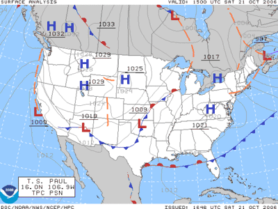
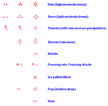
Surface weather analyses have special symbols that show frontal systems, cloud cover, precipitation, or other important information. For example, an H may represent high pressure, implying clear skies and relatively warm weather. An L, on the other hand, may represent low pressure, which frequently accompanies precipitation. Various symbols are used not just for frontal zones and other surface boundaries on weather maps, but also to depict the present weather at various locations on the weather map. Areas of precipitation help determine the frontal type and location.
History of surface analysis
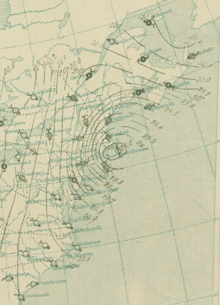
The use of weather charts in a modern sense began in the middle portion of the 19th century in order to devise a theory on storm systems.[3] The development of a telegraph network by 1845 made it possible to gather weather information from multiple distant locations quickly enough to preserve its value for real-time applications. The Smithsonian Institution developed its network of observers over much of the central and eastern United States between the 1840s and 1860s.[4] The U.S. Army Signal Corps inherited this network between 1870 and 1874 by an act of Congress, and expanded it to the west coast soon afterwards.
The weather data was at first less useful as a result of the different times at which weather observations were made. The first attempts at time standardization took hold in Great Britain by 1855. The entire United States did not finally come under the influence of time zones until 1905, when Detroit finally established standard time.[5] Other countries followed the lead of the United States in taking simultaneous weather observations, starting in 1873.[6] Other countries then began preparing surface analyses. The use of frontal zones on weather maps did not appear until the introduction of the Norwegian cyclone model in the late 1910s, despite Loomis' earlier attempt at a similar notion in 1841.[7] Since the leading edge of air mass changes bore resemblance to the military fronts of World War I, the term "front" came into use to represent these lines.[8]
Despite the introduction of the Norwegian cyclone model just after World War I, the United States did not formally analyze fronts on surface analyses until late 1942, when the WBAN Analysis Center opened in downtown Washington, D.C..[9] The effort to automate map plotting began in the United States in 1969,[10] with the process complete in the 1970s. Hong Kong completed their process of automated surface plotting by 1987.[11] By 1999, computer systems and software had finally become sophisticated enough to allow for the ability to underlay on the same workstation satellite imagery, radar imagery, and model-derived fields such as atmospheric thickness and frontogenesis in combination with surface observations to make for the best possible surface analysis. In the United States, this development was achieved when Intergraph workstations were replaced by n-AWIPS workstations.[12] By 2001, the various surface analyses done within the National Weather Service were combined into the Unified Surface Analysis, which is issued every six hours and combines the analyses of four different centers.[13] Recent advances in both the fields of meteorology and geographic information systems have made it possible to devise finely tailored weather maps. Weather information can quickly be matched to relevant geographical detail. For instance, icing conditions can be mapped onto the road network. This will likely continue to lead to changes in the way surface analyses are created and displayed over the next several years.[14] The pressureNET project is an ongoing attempt to gather surface pressure data using smartphones.
Station model used on weather maps

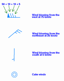
When analyzing a weather map, a station model is plotted at each point of observation. Within the station model, the temperature, dewpoint, wind speed and direction, atmospheric pressure, pressure tendency, and ongoing weather are plotted.[15] The circle in the middle represents cloud cover; fraction it is filled in represents the degree of overcast.[16] Outside the United States, temperature and dewpoint are plotted in degrees Celsius. The wind barb points in the direction from which the wind is coming. Each full flag on the wind barb represents 10 knots (19 km/h) of wind, each half flag represents 5 knots (9 km/h). When winds reach 50 knots (93 km/h), a filled in triangle is used for each 50 knots (93 km/h) of wind.[17] In the United States, rainfall plotted in the corner of the station model are in inches. The international standard rainfall measurement unit is the millimeter. Once a map has a field of station models plotted, the analyzing isobars (lines of equal pressure), isallobars (lines of equal pressure change), isotherms (lines of equal temperature), and isotachs (lines of equal wind speed) are drawn.[18] The abstract weather symbols were devised to take up the least room possible on weather maps.
Synoptic scale features
A synoptic scale feature is one whose dimensions are large in scale, more than several hundred kilometers in length.[19] Migratory pressure systems and frontal zones exist on this scale.
Pressure centers
Centers of surface high- and low-pressure areas that are found within closed isobars on a surface weather analysis are the absolute maxima and minima in the pressure field, and can tell a user in a glance what the general weather is in their vicinity. Weather maps in English-speaking countries will depict their highs as Hs and lows as Ls,[20] while Spanish-speaking countries will depict their highs as As and lows as Bs.[21]
Low pressure
Low-pressure systems, also known as cyclones, are located in minima in the pressure field. Rotation is inward at the surface and counterclockwise in the northern hemisphere as opposed to inward and clockwise in the southern hemisphere due to the Coriolis force. Weather is normally unsettled in the vicinity of a cyclone, with increased cloudiness, increased winds, increased temperatures, and upward motion in the atmosphere, which leads to an increased chance of precipitation. Polar lows can form over relatively mild ocean waters when cold air sweeps in from the ice cap. The relatively warmer water leads to upward convection, causing a low to form, and precipitation usually in the form of snow. Tropical cyclones and winter storms are intense varieties of low pressure. Over land, thermal lows are indicative of hot weather during the summer.[22]
High pressure
High-pressure systems, also known as anticyclones, rotate outward at the surface and clockwise in the northern hemisphere as opposed to outward and counterclockwise in the southern hemisphere. Under surface highs, sinking of the atmosphere slightly warms the air by compression, leading to clearer skies, winds that are lighter, and a reduced chance of precipitation.[23] The descending air is dry, hence less energy is required to raise its temperature. If high pressure persists, air pollution will build up due to pollutants trapped near the surface caused by the subsiding motion associated with the high.[24]
Fronts

Fronts in meteorology are the leading edges of air masses that have a density, air temperature, and humidity different from the air mass it is invading. When an air mass passes over an area, it is marked by changes in temperature, moisture, wind speed and direction, atmospheric pressure, and often a change in the precipitation pattern. The change is called a front, whether it be warm or cold. Cold fronts develop when cold air masses, usually moving equatorward from the polar region high pressure zones, interact with warm moist air of low pressure systems. The fronts develop at the leading edge of that cold air mass and wrap around (counter-clockwise in the northern hemisphere) about the low pressure zone. A polar front may form approximately along the equatorward edge of the high-level polar jet. Fronts are guided by winds aloft, but they normally move at lesser speeds than those winds. In the northern hemisphere, they usually travel from west to east, although they can move in a north-south direction as well as they may wrap around an associated low pressure zone. Movement is driven by the pressure gradient force (horizontal differences in atmospheric pressure) and the Coriolis force (caused by the Earth's rotation on its axis). Frontal zones can be distorted by such geographic features as mountains and large bodies of water.[13]
Cold front
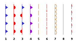
A cold front's location is at the leading edge of the temperature drop-off, which in an isotherm analysis shows up as the leading edge of the isotherm gradient, and it normally lies within a sharp surface trough. Cold fronts can move up to twice as fast as warm fronts and produce sharper changes in weather, since cold air is denser than warm air and rapidly lifts the warm air as the cold air moves in. Cold fronts are typically accompanied by a narrow band of showers and thunderstorms. On a weather map, the surface position of the cold front is marked with the symbol of a blue line of triangles/spikes (pips) pointing in the direction of travel, at the leading edge of the cooler air mass.[13]
Warm front
Warm fronts mark the position on the Earth's surface where a relatively warm body of air has displaced colder air. The temperature increase is located on the equatorward edge of the gradient in isotherms, and lies within broader low pressure troughs than is the case with cold fronts. Warm fronts move more slowly than do the cold fronts because cold air is denser, and harder to displace from the Earth's surface. This causes temperature differences across warm fronts to be broader in scale. The warm air mass overrides the cold air mass and temperature changes occur at higher altitudes before those at the surface. Clouds ahead of the warm front are mostly stratiform and rainfall gradually increases as the front approaches. Fog can also occur preceding a warm front passage. Clearing and warming is usually rapid after the passage of a warm front. If the warm air mass is unstable, mixing of the warm moist air will produce thunderstorms that are embedded among the stratiform clouds ahead of the front, and after frontal passage, thundershowers may continue. On weather maps, the surface location of a warm front is marked with a red line of half circles pointing in the direction of travel.[13]
Occluded front
1. cold front
2. warm front
3. stationary front
4. occluded front
5. surface trough
6. squall line
7. dry line
8. tropical wave
9. Trowal
An occluded front is formed during the process of cyclogenesis when a cold front overtakes a warm front.[25] The cold and warm fronts curve naturally poleward into the point of occlusion, which is also known as the triple point in meteorology.[26] It lies within a sharp trough, but the air mass behind the boundary can be either warm or cold. In a cold occlusion, the air mass overtaking the warm front is cooler than the cool air ahead of the warm front, and plows under both air masses. In a warm occlusion, the air mass overtaking the warm front is not as cool as the cold air ahead of the warm front, and rides over the colder air mass while lifting the warm air. A wide variety of weather can be found along an occluded front, with thunderstorms possible, but usually their passage is associated with a drying of the air mass. Occluded fronts are indicated on a weather map by a purple line with alternating half-circles and triangles pointing in direction of travel.[13] Occluded fronts usually form around mature low pressure areas.
The trowal is the projection on the Earth's surface of a tongue of warm air aloft, such as may be formed during the occlusion process of a depression.[27]
Stationary fronts and shearlines
A stationary front is a non-moving boundary between two different air masses, neither of which is strong enough to replace the other. They tend to remain in the same area for long periods of time, usually moving in waves.[28] There is normally a broad temperature gradient behind the boundary with more widely spaced isotherms. A wide variety of weather can be found along a stationary front, but usually clouds and prolonged precipitation are found there. Stationary fronts will either dissipate after several days or devolve into shear lines, but can change into a cold or warm front if conditions aloft change causing a driving of one air mass or the other. Stationary fronts are marked on weather maps with alternating red half-circles and blue spikes pointing in opposite directions, indicating no significant movement.
When stationary fronts become smaller in scale, degenerating to a narrow zone where wind direction changes over a short distance, they become known as shear lines.[29] If the shear line becomes active with thunderstorms, it may support formation of a tropical storm or a regeneration of the feature back into a stationary front. A shear line is depicted as a line of red dots and dashes.[13]
Mesoscale features
Mesoscale features are smaller than synoptic scale systems like fronts, but larger than storm-scale systems like thunderstorms. Horizontal dimensions generally range from over ten kilometres to several hundred kilometres.[30]
Dry line
The dry line is the boundary between dry and moist air masses east of mountain ranges with similar orientation to the Rockies, depicted at the leading edge of the dew point, or moisture, gradient. Near the surface, warm moist air that is denser than warmer, dryer air wedges under the drier air in a manner similar to that of a cold front wedging under warmer air.[31] When the warm moist air wedged under the drier mass heats up, it becomes less dense and rises and sometimes forms thunderstorms.[32] At higher altitudes, the warm moist air is less dense than the cooler, drier air and the boundary slope reverses. In the vicinity of the reversal aloft, severe weather is possible, especially when a triple point is formed with a cold front.
During daylight hours, drier air from aloft drifts down to the surface, causing an apparent movement of the dryline eastward. At night, the boundary reverts to the west as there is no longer any solar heating to help mix the lower atmosphere.[33] If enough moisture converges upon the dryline, it can be the focus of afternoon and evening thunderstorms.[34] A dry line is depicted on United States surface analyses as a brown line with scallops, or bumps, facing into the moist sector. Dry lines are one of the few surface fronts where the special shapes along the drawn boundary do not necessarily reflect the boundary's direction of motion.[35]
Outflow boundaries and squall lines

Organized areas of thunderstorm activity not only reinforce pre-existing frontal zones, but they can outrun cold fronts. This outrunning occurs in a pattern where the upper level jet splits into two streams. The resultant mesoscale convective system (MCS) forms at the point of the upper level split in the wind pattern at the area of the best low-level inflow. The convection then moves east and equatorward into the warm sector, parallel to low-level thickness lines. When the convection is strong and linear or curved, the MCS is called a squall line, with the feature placed at the leading edge where the significant wind shifts and pressure rises.[36] Even weaker and less organized areas of thunderstorms will lead to locally cooler air and higher pressures, and outflow boundaries exist ahead of this type of activity, "SQLN" or "SQUALL LINE", while outflow boundaries are depicted as troughs with a label of "OUTFLOW BOUNDARY" or "OUTFLOW BNDRY".
Sea and land breeze fronts
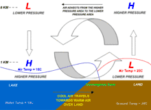
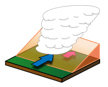
Sea breeze fronts occur on sunny days when the landmass warms the air above it to a temperature above the water temperature. Similar boundaries from downwind on lakes and rivers during the day, as well as offshore landmasses at night. Since the specific heat of water is so high, there is little diurnal temperature change in bodies of water, even on the sunniest days. The water temperature varies less than 1 °C (1.8 °F). By contrast, the land, with a lower specific heat, can vary several degrees in a matter of hours.[37]
During the afternoon, air pressure decreases over the land as the warmer air rises. The relatively cooler air over the sea rushes in to replace it. The result is a relatively cool onshore wind. This process usually reverses at night where the water temperature is higher relative to the landmass, leading to an offshore land breeze. However, if water temperatures are colder than the land at night, the sea breeze may continue, only somewhat abated. This is typically the case along the California coast, for example.
If enough moisture exists, thunderstorms can form along sea breeze fronts that then can send out outflow boundaries. This causes chaotic wind/pressure regimes if the steering flow is weak. Like all other surface features, sea breeze fronts lie inside troughs of low pressure.
See also
- Bowditch's American Practical Navigator
- Extratropical cyclone
- Frontolysis
- Outline of meteorology
- Ridge (meteorology)
References
- Air Apparent: How Meteorologists Learned to Map, Predict, and Dramatize Weather. University of Chicago PressChicago: 1999.
- Eric R. Miller. American Pioneers in Meteorology. Retrieved on 2007-04-18.
- Human Intelligence.Francis Galton. Retrieved on 2007-04-18.
- Frank Rives Millikan. Smithsonian Institution. Joseph Henry: Father of the Weather Service. Retrieved on 2006-10-22. Archived October 20, 2006, at the Wayback Machine
- WebExhibits. Daylight Saving Time. Retrieved on 2007-06-24.
- NOAA. An Expanding Presence. Retrieved on 2007-05-05.
- David M. Schultz. Perspectives on Fred Sanders's Research on Cold Fronts, 2003, revised, 2004, 2006, p. 5. Retrieved on 2006-07-14.
- Bureau of Meteorology. Air Masses and Weather Maps. Retrieved on 2006-10-22.
- Hydrometeorological Prediction Center. A Brief History of the Hydrometeorological Prediction Center. Retrieved on 2007-05-05.
- ESSA. Prospectus for an NMC Digital Facsimile Incoder Mapping Program. Retrieved on 2007-05-05.
- Hong Kong Observatory. The Hong Kong Observatory Computer System and Its Applications. Archived 2006-12-31 at the Wayback Machine Retrieved on 2007-05-05.
- Hydrometeorological Prediction Center. Hydrometeorological Prediction Center 1999 Accomplishment Report. Retrieved on 2007-05-05.
- David Roth. Hydrometeorological Prediction Center. Unified Surface Analysis Manual. Retrieved on 2006-10-22.
- Saseendran S. A., Harenduprakash L., Rathore L. S. and Singh S. V. A GIS application for weather analysis and forecasting. Retrieved on 2007-05-05.
- National Weather Service. Station Model Example. Retrieved on 2007-04-29. Archived October 25, 2007, at the Wayback Machine
- Dr Elizabeth R. Tuttle. Weather Maps. Archived 2008-07-09 at the Wayback Machine Retrieved on 2007-05-10.
- American Meteorological Society. Selected DataStreme Atmosphere Weather Map Symbols. Retrieved on 2007-05-10.
- CoCoRAHS. INTRODUCTION TO DRAWING ISOPLETHS. Retrieved on 2007-04-29. Archived April 28, 2007, at the Wayback Machine
- Glossary of meteorology. Synoptic scale. Archived 2007-08-11 at the Wayback Machine Retrieved on 2007-05-10.
- Weather Doctor. Weather's Highs and Lows: Part 1 The High.
- Agencia Estatal de Meteorología. Meteorología del aeropuerto de La Palma..
- BBC Weather. Weather Basics - Low Pressure. Retrieved on 2007-05-05.
- BBC Weather. High Pressure. Retrieved on 2007-05-05.
- United Kingdom School System. Pressure, Wind and Weather Systems. Archived 2007-09-27 at the Wayback Machine Retrieved on 2007-05-05.
- University of Illinois. Occluded Front. Retrieved on 2006-10-22.
- National Weather Service Office, Norman, Oklahoma. Triple Point. Retrieved on 2006-10-22. Archived October 9, 2006, at the Wayback Machine
- "Trowal". World Meteorological Organisation. Eumetcal. Archived from the original on 2014-03-31. Retrieved 2013-08-28.
- University of Illinois. Stationary Front. Retrieved on 2006-10-22.
- Glossary of Meteorology. Shear Line. Archived 2007-03-14 at the Wayback Machine Retrieved on 2006-10-22.
- Fujita, T. T., 1986. Mesoscale classifications: their history and their application to forecasting. Mesoscale Meteorology and Forecasting. American Meteorological Society, Boston, p. 18–35.
- Huaqing Cai. Dryline cross section. Archived 2008-01-20 at the Wayback Machine Retrieved on 2006-12-05.
- "Lecture 3". Archived from the original on 27 September 2007.
- Lewis D. Grasso. A Numerical Simulation of Dryline Sensitivity to Soil Moisture. Retrieved on 2007-05-10.
- Glossary of Meteorology. Lee Trough. Archived 2011-09-19 at the Wayback Machine Retrieved on 2006-10-22.
- University of Illinois. Dry Line: A Moisture Boundary. Retrieved on 2006-10-22.
- Office of the Federal Coordinator for Meteorology.Chapter 2: Definitions. Archived 2009-05-06 at the Wayback Machine Retrieved on 2006-10-22.
- Glossary of Meteorology. Sea Breeze. Archived 2007-03-14 at the Wayback Machine Retrieved on 2006-10-22.
External links
| Wikimedia Commons has media related to Atmospheric fronts. |