Smoothness
In mathematical analysis, the smoothness of a function is a property measured by the number of continuous derivatives it has over some domain.[1][2] At the very minimum, a function could be considered "smooth" if it is differentiable everywhere (hence continuous).[3] At the other end, it might also possess derivatives of all orders in its domain, in which case it is referred to as a C-infinity function (or function).[4]


Differentiability classes
Differentiability class is a classification of functions according to the properties of their derivatives. It's a measure of the highest order of derivative that exist for a function.
Consider an open set on the real line and a function f defined on that set with real values. Let k be a non-negative integer. The function f is said to be of (differentiability) class Ck if the derivatives f′, f′′, ..., f(k) exist and are continuous (continuity is implied by differentiability for all the derivatives except for f(k)). The function f is said to be of class C∞, or smooth, if it has derivatives of all orders.[5] The function f is said to be of class Cω, or analytic, if f is smooth and if its Taylor series expansion around any point in its domain converges to the function in some neighborhood of the point. Cω is thus strictly contained in C∞. Bump functions are examples of functions in C∞ but not in Cω.
To put it differently, the class C0 consists of all continuous functions. The class C1 consists of all differentiable functions whose derivative is continuous; such functions are called continuously differentiable. Thus, a C1 function is exactly a function whose derivative exists and is of class C0. In general, the classes Ck can be defined recursively by declaring C0 to be the set of all continuous functions, and declaring Ck for any positive integer k to be the set of all differentiable functions whose derivative is in Ck−1. In particular, Ck is contained in Ck−1 for every k > 0, and there are examples to show that this containment is strict (Ck ⊊ Ck−1). C∞, the class of infinitely differentiable functions, is the intersection of the sets Ck—as k varies over the non-negative integers (i.e. from 0 to ∞).
Examples
.svg.png)
.svg.png)


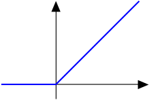
The function

is continuous, but not differentiable at x = 0, so it is of class C0, but not of class C1.
The function

is differentiable, with derivative

Because oscillates as x → 0, is not continuous at zero. Therefore, is differentiable but not of class C1. Moreover, if one takes (x ≠ 0) in this example, it can be used to show that the derivative function of a differentiable function can be unbounded on a compact set and, therefore, that a differentiable function on a compact set may not be locally Lipschitz continuous.


The functions

where k is even, are continuous and k times differentiable at all x. But at x = 0 they are not (k + 1) times differentiable, so they are of class Ck, but not of class Cj where j > k.
The exponential function is analytic, and hence falls into the class Cω. The trigonometric functions are also analytic wherever they are defined.
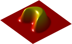
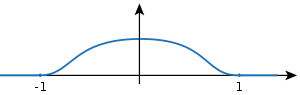
The bump function

is smooth, so of class C∞, but it is not analytic at x = ±1, and hence is not of class Cω. The function f is an example of a smooth function with compact support.
Multivariate differentiability classes
A function defined on an open set of is said[6] to be of class on , for a positive integer , if all partial derivatives


exist and are continuous, for every non-negative integers, such that , and every . The function is said to be of class or if it is continuous on .


A function , defined on an open set of , is said to be of class on , for a positive integer , if all of its components


are of class , where are the natural projections defined by . It is said to be of class or if it is continuous, or equivalently, if all components are continuous, on .


The space of Ck functions
Let D be an open subset of the real line. The set of all Ck real-valued functions defined on D is a Fréchet vector space, with the countable family of seminorms

where K varies over an increasing sequence of compact sets whose union is D, and m = 0, 1, ..., k.
The set of C∞ functions over D also forms a Fréchet space. One uses the same seminorms as above, except that m is allowed to range over all non-negative integer values.
The above spaces occur naturally in applications where functions having derivatives of certain orders are necessary; however, particularly in the study of partial differential equations, it can sometimes be more fruitful to work instead with the Sobolev spaces.
Parametric continuity
The terms parametric continuity and geometric continuity (Gn) were introduced by Brian Barsky, to show that the smoothness of a curve could be measured by removing restrictions on the speed, with which the parameter traces out the curve.[7][8][9]
Parametric continuity is a concept applied to parametric curves, which describes the smoothness of the parameter's value with distance along the curve.
Definition
A (parametric) curve is said to be of class Ck, if exists and is continuous on , where derivatives at the end-points are taken to be one sided derivatives (i.e., at from the right, and at from the left).


As a practical application of this concept, a curve describing the motion of an object with a parameter of time must have C1 continuity—for the object to have finite acceleration. For smoother motion, such as that of a camera's path while making a film, higher orders of parametric continuity are required.
Order of continuity

The various order of parametric continuity can be described as follows:[10]
- C0: Curves are continuous
- C1: First derivatives are continuous
- C2: First and second derivatives are continuous
- Cn: First through nth derivatives are continuous
Geometric continuity
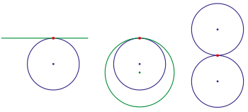

pencil of conic sections with G2-contact: p fix, variable

(: circle,: ellipse, : parabola, : hyperbola)


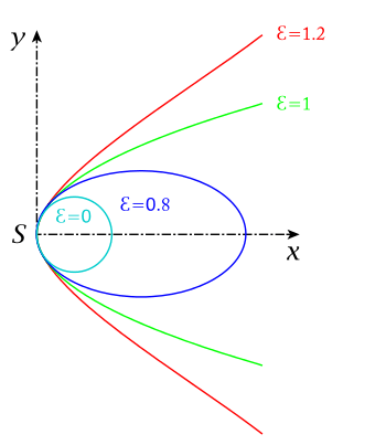
The concept of geometrical or geometric continuity was primarily applied to the conic sections (and related shapes) by mathematicians such as Leibniz, Kepler, and Poncelet. The concept was an early attempt at describing, through geometry rather than algebra, the concept of continuity as expressed through a parametric function.[11]
The basic idea behind geometric continuity was that the five conic sections were really five different versions of the same shape. An ellipse tends to a circle as the eccentricity approaches zero, or to a parabola as it approaches one; and a hyperbola tends to a parabola as the eccentricity drops toward one; it can also tend to intersecting lines. Thus, there was continuity between the conic sections. These ideas led to other concepts of continuity. For instance, if a circle and a straight line were two expressions of the same shape, perhaps a line could be thought of as a circle of infinite radius. For such to be the case, one would have to make the line closed by allowing the point to be a point on the circle, and for and to be identical. Such ideas were useful in crafting the modern, algebraically defined, idea of the continuity of a function and of (see projectively extended real line for more).[11]


Smoothness of curves and surfaces
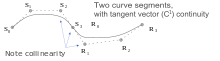
A curve or surface can be described as having Gn continuity, with n being the increasing measure of smoothness. Consider the segments either side of a point on a curve:
- G0: The curves touch at the join point.
- G1: The curves also share a common tangent direction at the join point.
- G2: The curves also share a common center of curvature at the join point.
In general, Gn continuity exists if the curves can be reparameterized to have Cn (parametric) continuity.[12][13] A reparametrization of the curve is geometrically identical to the original; only the parameter is affected.
Equivalently, two vector functions f(t) and g(t) have Gn continuity if f(n)(t) ≠ 0 and f(n)(t) ≡ kg(n)(t), for a scalar k > 0 (i.e., if the direction, but not necessarily the magnitude, of the two vectors is equal).
While it may be obvious that a curve would require G1 continuity to appear smooth, for good aesthetics, such as those aspired to in architecture and sports car design, higher levels of geometric continuity are required. For example, reflections in a car body will not appear smooth unless the body has G2 continuity.
A rounded rectangle (with ninety degree circular arcs at the four corners) has G1 continuity, but does not have G2 continuity. The same is true for a rounded cube, with octants of a sphere at its corners and quarter-cylinders along its edges. If an editable curve with G2 continuity is required, then cubic splines are typically chosen; these curves are frequently used in industrial design.
Smoothness of piecewise defined curves and surfaces
Other concepts
Relation to analyticity
While all analytic functions are "smooth" (i.e. have all derivatives continuous) on the set on which they are analytic, examples such as bump functions (mentioned above) show that the converse is not true for functions on the reals: there exist smooth real functions that are not analytic. Simple examples of functions that are smooth but not analytic at any point can be made by means of Fourier series; another example is the Fabius function. Although it might seem that such functions are the exception rather than the rule, it turns out that the analytic functions are scattered very thinly among the smooth ones; more rigorously, the analytic functions form a meagre subset of the smooth functions. Furthermore, for every open subset A of the real line, there exist smooth functions that are analytic on A and nowhere else.
It is useful to compare the situation to that of the ubiquity of transcendental numbers on the real line. Both on the real line and the set of smooth functions, the examples we come up with at first thought (algebraic/rational numbers and analytic functions) are far better behaved than the majority of cases: the transcendental numbers and nowhere analytic functions have full measure (their complements are meagre).
The situation thus described is in marked contrast to complex differentiable functions. If a complex function is differentiable just once on an open set, it is both infinitely differentiable and analytic on that set.
Smooth partitions of unity
Smooth functions with given closed support are used in the construction of smooth partitions of unity (see partition of unity and topology glossary); these are essential in the study of smooth manifolds, for example to show that Riemannian metrics can be defined globally starting from their local existence. A simple case is that of a bump function on the real line, that is, a smooth function f that takes the value 0 outside an interval [a,b] and such that

Given a number of overlapping intervals on the line, bump functions can be constructed on each of them, and on semi-infinite intervals (-∞, c] and [d, +∞) to cover the whole line, such that the sum of the functions is always 1.
From what has just been said, partitions of unity don't apply to holomorphic functions; their different behavior relative to existence and analytic continuation is one of the roots of sheaf theory. In contrast, sheaves of smooth functions tend not to carry much topological information.
Smooth functions on and between manifolds
Given a smooth manifold , dimension m, with atlas , then a map is smooth on M if for all there exists a chart , such that the pullback of by , denoted is smooth as a function from to in a neighborhood of (all partial derivatives up to a given order are continuous). Note that smoothness can be checked with respect to any preferred chart about p in the atlas, since the smoothness requirements on the transition functions between charts ensure that if is smooth about p in one chart it will be smooth about p in any other chart of the atlas. If instead is a map from to an n-dimensional manifold , then F is smooth if, for every p ∈ M, there is a chart about p in , and a chart about in with , such that is smooth as a function from Rm to Rn.


Smooth maps between manifolds induce linear maps between tangent spaces: for , at each point the pushforward (or differential) maps tangent vectors at p to tangent vectors at F(p): , and on the level of the tangent bundle, the pushforward is a vector bundle homomorphism: . The dual to the pushforward is the pullback, which "pulls" covectors on back to covectors on , and k-forms to k-forms: . In this way smooth functions between manifolds can transport local data, like vector fields and differential forms, from one manifold to another, or down to Euclidean space where computations like integration are well understood.


Preimages and pushforwards along smooth functions are, in general, not manifolds without additional assumptions. Preimages of regular points (that is, if the differential does not vanish on the preimage) are manifolds; this is the preimage theorem. Similarly, pushforwards along embeddings are manifolds.[14]
Smooth functions between subsets of manifolds
There is a corresponding notion of smooth map for arbitrary subsets of manifolds. If f : X → Y is a function whose domain and range are subsets of manifolds X ⊂ M and Y ⊂ N respectively. f is said to be smooth if for all x ∈ X there is an open set U ⊂ M with x ∈ U and a smooth function F : U → N such that F(p) = f(p) for all p ∈ U ∩ X.
See also
- Non-analytic smooth function
- Quasi-analytic function
- Singularity (mathematics)
- Sinuosity
- Smooth scheme
- Smooth number (number theory)
- Smoothing
- Spline
References
- "The Definitive Glossary of Higher Mathematical Jargon — Smooth". Math Vault. 2019-08-01. Retrieved 2019-12-13.
- Weisstein, Eric W. "Smooth Function". mathworld.wolfram.com. Retrieved 2019-12-13.
- "Smooth (mathematics)". TheFreeDictionary.com. Retrieved 2019-12-13.
- "Smooth function - Encyclopedia of Mathematics". www.encyclopediaofmath.org. Retrieved 2019-12-13.
- Warner, Frank W. (1983). Foundations of Differentiable Manifolds and Lie Groups. Springer. p. 5 [Definition 1.2]. ISBN 978-0-387-90894-6.
- Henri Cartan (1977). Cours de calcul différentiel. Paris: Hermann.
- Barsky, Brian A. (1981). The Beta-spline: A Local Representation Based on Shape Parameters and Fundamental Geometric Measures (Ph.D.). University of Utah, Salt Lake City, Utah.
- Brian A. Barsky (1988). Computer Graphics and Geometric Modeling Using Beta-splines. Springer-Verlag, Heidelberg. ISBN 978-3-642-72294-3.
- Richard H. Bartels; John C. Beatty; Brian A. Barsky (1987). An Introduction to Splines for Use in Computer Graphics and Geometric Modeling. Morgan Kaufmann. Chapter 13. Parametric vs. Geometric Continuity. ISBN 978-1-55860-400-1.
- van de Panne, Michiel (1996). "Parametric Curves". Fall 1996 Online Notes. University of Toronto, Canada.
- Taylor, Charles (1911). . In Chisholm, Hugh (ed.). Encyclopædia Britannica. 11 (11th ed.). Cambridge University Press. pp. 674–675.
- Barsky, Brian A.; DeRose, Tony D. (1989). "Geometric Continuity of Parametric Curves: Three Equivalent Characterizations". IEEE Computer Graphics and Applications. 9 (6): 60–68. doi:10.1109/38.41470.
- Hartmann, Erich (2003). "Geometry and Algorithms for Computer Aided Design" (PDF). Technische Universität Darmstadt. p. 55.
- Guillemin, Victor; Pollack, Alan (1974). Differential Topology. Englewood Cliffs: Prentice-Hall. ISBN 0-13-212605-2.CS1 maint: ref=harv (link)