Cubic function

The roots, stationary points, inflection point and concavity of a cubic polynomial x³ − 3x² − 144x + 432 (black line) and its first and second derivatives (red and blue).

The critical points of a cubic function are its stationary points, that is the points where the slope of the function is zero. Thus the critical points of a cubic function f defined by

f(x) = ax³ + bx² + cx + d,

occur at values of x such that the derivative

${\displaystyle 3ax^{2}+2bx+c=0}$

of the cubic function is zero.

The solutions of this equation are the x-values of the critical points and are given, using the quadratic formula, by

${\displaystyle x_{\text{critical}}={\frac {-b\pm {\sqrt {b^{2}-3ac}}}{3a}}.}$

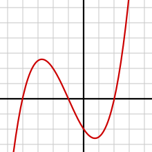
The sign of the expression inside the square root determines the number of critical points. If it is positive, then there are two critical points, one is a local maximum, and the other is a local minimum. If b² – 3ac = 0, then there is only one critical point, which is an inflection point. If b² – 3ac < 0, then there are no (real) critical points. In the two latter cases, that is, if b² – 3ac is nonpositive, the cubic function is strictly monotonic. See the figure for an example of the case Δ₀ > 0.

The inflection point of a function is where that function changes concavity. An inflection point occurs when the second derivative is zero, and the third derivative is nonzero. Thus a cubic function has always a single inflection point, which occurs at

${\displaystyle x_{\text{inflection}}=-{\frac {b}{3a}}.}$

Cubic functions of the form ${\displaystyle y=x^{3}+px.}$
The graph of any cubic function is similar to such a curve.

The graph of a cubic function is an example of a cubic curve. (Many cubic curves are not graphs of functions.)

Although cubic functions depend on four parameters, their graph can have only very few shapes. In fact, the graph of a cubic function is always similar to the graph of a function of the form

${\displaystyle y=x^{3}+px.}$

This similarity can be built as the composition of translations parallel to the coordinates axes, a homothecy (uniform scaling), and, possibly, a reflection (mirror image) with respect to the y-axis. A further non-uniform scaling can transform the graph into the graph of one among the three cubic functions

${\displaystyle {\begin{aligned}y&=x^{3}+x\\y&=x^{3}\\y&=x^{3}-x.\end{aligned}}}$

This means that there are only three graphs of cubic functions up to an affine transformation.

The above geometric transformations can be built in the following way, when starting from a general cubic function ${\displaystyle y=ax^{3}+bx^{2}+cx+d.}$

Firstly, if a < 0, the change of variable x → –x allows supposing a > 0. After this change of variable, the new graph is the mirror image of the previous one, with respect of the y-axis.

Then, the change of variable x = x₁ – b/3a provides a function of the form

${\displaystyle y=ax_{1}^{3}+px+q.}$

This corresponds to a translation parallel to the x-axis.

The change of variable y = y₁ + q corresponds to a translation with respect to the y-axis, and gives a function of the form

${\displaystyle y_{1}=ax_{1}^{3}+px.}$

The change of variable ${\displaystyle \textstyle x_{1}={\frac {x_{2}}{\sqrt {a}}},y_{1}={\frac {y_{2}}{\sqrt {a}}}}$ corresponds to a uniform scaling, and give, after division by ${\displaystyle {\sqrt {a}},}$ a function of the form

${\displaystyle y_{2}=x_{2}^{3}+px,}$

which is the simplest form that can be obtained by a similarity.

Then, if p ≠ 0, the non-uniform scaling ${\displaystyle \textstyle x_{2}=x_{3}{\sqrt {|p|}},\quad y_{2}=y_{3}{\sqrt {|p|^{3}}}}$ gives, after division by ${\displaystyle \textstyle {\sqrt {|p|^{3}}},}$

${\displaystyle y_{3}=x_{3}+x\operatorname {sign} (p),}$

where ${\displaystyle \operatorname {sign} (p)}$ has the value 1 or –1, depending on the sign of p. If one defines ${\displaystyle \operatorname {sign} (0)=0,}$ the latter form of the function applies to all cases.

For a cubic function of the form ${\displaystyle y=x^{3}+px,}$ the inflection point is thus the origin. As such a function is an odd function, its graph is symmetric with respect to the inflection point, and invariant under a rotation of a half turn around the inflection point. As these properties are invariant by similarity, the following is true for all cubic functions.

The graph of a cubic function is symmetric with respect to its inflection point, and is invariant under a rotation of a half turn around the inflection point.

The points P₁, P₂, and P₃ (in blue) are collinear and belong to the graph of x³ + 3/2x² − 5/2x + 5/4. The points T₁, T₂, and T₃ (in red) are the intersections of the (dotted) tangent lines to the graph at these points with the graph itself. They are collinear too.

The tangent lines to the graph of a cubic function at three collinear points intercept the cubic again at collinear points.[1] This can be seen as follows.

As this property is invariant under a rigid motion, one may suppose that the function has the form

${\displaystyle f(x)=x^{3}+px.}$

If α is a real number, then the tangent to the graph of f at the point (α, f(α)) is the line

{(x, f(α) + (x − α)f ′(α)) : x ∈ R}.

So, the intersection point between this line and the graph of f can be obtained solving the equation f(x) = f(α) + (x − α)f ′(α), that is

${\displaystyle x^{3}+px=\alpha ^{3}+p\alpha +(x-\alpha )(3\alpha ^{2}+p),}$

which can be rewritten

${\displaystyle x^{3}-3\alpha ^{2}x+2\alpha ^{3}=0,}$

and factorized as

${\displaystyle (x-\alpha )^{2}(x+2\alpha )=0.}$

So, the tangent intercepts the cubic at

${\displaystyle (-2\alpha ,-8\alpha ^{3}-2p\alpha )=(-2\alpha ,-8f(\alpha )-10p\alpha ).}$

So, the function that maps a point (x, y) of the graph to the other point where the tangent intercepts the graph is

${\displaystyle (x,y)\mapsto (-2x,-8y-10px).}$

This is an affine transformation that transforms collinear points into collinear points. This proves the claimed result.

Given the values of a function and its derivative at two points, there is exactly one cubic function that has the same four values, which is called a cubic Hermite spline.

There are two standard ways for using this fact. Firstly, if one knows, for example by physical measurement, the values of a function and its derivative at some sampling points, one can interpolate the function with a continuously differentiable function, which is a piecewise cubic function.

If the value of a function is known at several points, cubic interpolation consists in approximating the function by a continuously differentiable function, which is piecewise cubic. For having a uniquely defined interpolation, two more constraints must be added, such as the values of the derivatives at the endpoints, or a zero curvature at the endpoints.

Wikimedia Commons has media related to Cubic functions.

• Hazewinkel, Michiel, ed. (2001) [1994], "Cardano formula", Encyclopedia of Mathematics, Springer Science+Business Media B.V. / Kluwer Academic Publishers, ISBN 978-1-55608-010-4
• History of quadratic, cubic and quartic equations on MacTutor archive.