SymPy
SymPy is an open-source Python library for symbolic computation. It provides computer algebra capabilities either as a standalone application, as a library to other applications, or live on the web as SymPy Live or SymPy Gamma. SymPy is simple to install and to inspect because it is written entirely in Python with few dependencies.[2][3][4] This ease of access combined with a simple and extensible code base in a well known language make SymPy a computer algebra system with a relatively low barrier to entry.
| Developer(s) | SymPy Development Team |
|---|---|
| Initial release | 2007 |
| Stable release | 1.6[1]
/ 24 May 2020 |
| Repository | |
| Written in | Python |
| Operating system | Cross-platform |
| Type | Computer algebra system |
| License | New BSD License |
| Website | www |
SymPy includes features ranging from basic symbolic arithmetic to calculus, algebra, discrete mathematics and quantum physics. It is capable of formatting the result of the computations as LaTeX code.[2][3]
SymPy is free software and is licensed under New BSD License. The lead developers are Ondřej Čertík and Aaron Meurer. It was started in 2005 by Ondřej Čertík.[5]
Features
The SymPy library is split into a core with many optional modules.
Currently, the core of SymPy has around 260,000 lines of code[6] (also includes a comprehensive set of self-tests: over 100,000 lines in 350 files as of version 0.7.5), and its capabilities include:[2][3][7][8][9]
Core capabilities
- Basic arithmetic: *, /, +, -, **
- Simplification
- Expansion
- Functions: trigonometric, hyperbolic, exponential, roots, logarithms, absolute value, spherical harmonics, factorials and gamma functions, zeta functions, polynomials, hypergeometric, special functions, ...
- Substitution
- Arbitrary precision integers, rationals and floats
- Noncommutative symbols
- Pattern matching
Polynomials
- Basic arithmetic: division, gcd, ...
- Factorization
- Square-free factorization
- Gröbner bases
- Partial fraction decomposition
- Resultants
Calculus
- Limits
- Differentiation
- Integration: Implemented Risch–Norman heuristic
- Taylor series (Laurent series)
Solving equations
- Polynomials
- Systems of equations
- Algebraic equations
- Differential equations
- Difference equations
Discrete math
- Binomial coefficients
- Summations
- Products
- Number theory: generating prime numbers, primality testing, integer factorization, ...
- Logic expressions
- Logical Reasoning[10]
Matrices
- Basic arithmetic
- Eigenvalues/eigenvectors
- Determinants
- Inversion
- Solving
Geometry
- Points, lines, rays, segments, ellipses, circles, polygons, ...
- Intersections
- Tangency
- Similarity
Plotting
Note, plotting requires the external matplotlib or Pyglet module.
- Coordinate models
- Plotting Geometric Entities
- 2D and 3D
- Interactive interface
- Colors
- Animations
Physics
Statistics
Combinatorics
- Permutations
- Combinations
- Partitions
- Subsets
- Permutation group: Polyhedral, Rubik, Symmetric, ...
- Prufer sequence and Gray Codes
Printing
- Pretty-printing: ASCII/Unicode pretty-printing, LaTeX
- Code generation: C, Fortran, Python
Related projects
- SageMath: an open source alternative to Mathematica, Maple, MATLAB, and Magma (SymPy is included in Sage)
- SymEngine: a rewriting of SymPy's core in C++, in order to increase its performance. Work is currently in progress to make SymEngine the underlying engine of Sage too.
- mpmath: a Python library for arbitrary-precision floating-point arithmetic
- SympyCore: another Python computer algebra system
- SfePy: Software for solving systems of coupled partial differential equations (PDEs) by the finite element method in 1D, 2D and 3D.
- GAlgebra: Geometric algebra module (previously sympy.galgebra).
- Quameon: Quantum Monte Carlo in Python.
- Lcapy: Experimental Python package for teaching linear circuit analysis.
- LaTeX Expression project: Easy LaTeX typesetting of algebraic expressions in symbolic form with automatic substitution and result computation.
- Symbolic statistical modeling: Adding statistical operations to complex physical models.
- Diofant: a fork of the SymPy, started by Sergey B Kirpichev
Dependencies
Since version 1.0, SymPy has the mpmath package as a dependency.
There are several optional dependencies that can enhance its capabilities:
- gmpy: If gmpy is installed, the SymPy's polynomial module will automatically use it for faster ground types. This can provide a several times boost in performance of certain operations.
- matplotlib: If matplotlib is installed, SymPy can use it for plotting.
- Pyglet: Alternative plotting package.
Usage examples
Pretty-printing
Sympy allows outputs to be formatted into a more appealing format through the pprint function. Alternatively, the init_printing() method will enable pretty-printing, so pprint need not be called. Pretty-printing will use unicode symbols when available in the current environment, otherwise it will fall back to ASCII characters.
>>> from sympy import pprint, init_printing, Symbol, sin, cos, exp, sqrt, series, Integral, Function
>>>
>>> x = Symbol("x")
>>> y = Symbol("y")
>>> f = Function('f')
>>> # pprint will default to unicode if available
>>> pprint( x**exp(x) )
 ⎛ x⎞
 ⎝ℯ ⎠
x
>>> # An output without unicode
>>> pprint(Integral(f(x), x), use_unicode=False)
  /
 |
 | f(x) dx
 |
/
>>> # Compare with same expression but this time unicode is enabled
>>> pprint(Integral(f(x), x), use_unicode=True)
⌠
⎮ f(x) dx
⌡
>>> # Alternatively, you can call init_printing() once and pretty-print without the pprint function.
>>> init_printing()
>>> sqrt(sqrt(exp(x)))
   ____
4 ╱  x
╲╱  ℯ
>>> (1/cos(x)).series(x, 0, 10)
     2      4       6        8
    x    5⋅x    61⋅x    277⋅x     ⎛ 10⎞
1 + ── + ──── + ───── + ────── + O⎝x  ⎠
    2     24     720     8064
Expansion
>>> from sympy import init_printing, Symbol, expand
>>> init_printing()
>>>
>>> a = Symbol('a')
>>> b = Symbol('b')
>>> e = (a + b)**5
>>> e
       5
(a + b)
>>> e.expand()
 5     4        3  2      2  3       4    5
a  + 5⋅a ⋅b + 10⋅a ⋅b  + 10⋅a ⋅b  + 5⋅a⋅b  + b
Arbitrary-precision example
>>> from sympy import Rational, pprint
>>> e = 2**50 / Rational(10)**50
>>> pprint(e)
1/88817841970012523233890533447265625
Differentiation
>>> from sympy import init_printing, symbols, ln, diff
>>> init_printing()
>>> x, y = symbols('x y')
>>> f = x**2 / y + 2 * x - ln(y)
>>> diff(f, x)
 2⋅x
 ─── + 2
  y
>>> diff(f, y)
    2
   x    1
 - ── - ─
    2   y
   y
>>> diff(diff(f, x), y)
 -2⋅x
 ────
   2
  y
Plotting
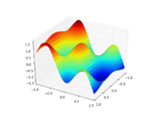
>>> from sympy import symbols, cos
>>> from sympy.plotting import plot3d
>>> x, y = symbols('x y')
>>> plot3d(cos(x*3)*cos(y*5)-y, (x, -1, 1), (y, -1, 1))
<sympy.plotting.plot.Plot object at 0x3b6d0d0>
Limits
>>> from sympy import init_printing, Symbol, limit, sqrt, oo
>>> init_printing()
>>>
>>> x = Symbol('x')
>>> limit(sqrt(x**2 - 5*x + 6) - x, x, oo)
-5/2
>>> limit(x*(sqrt(x**2 + 1) - x), x, oo)
1/2
>>> limit(1/x**2, x, 0)
∞
>>> limit(((x - 1)/(x + 1))**x, x, oo)
 -2
ℯ
Differential equations
>>> from sympy import init_printing, Symbol, Function, Eq, dsolve, sin, diff
>>> init_printing()
>>>
>>> x = Symbol("x")
>>> f = Function("f")
>>>
>>> eq = Eq(f(x).diff(x), f(x))
>>> eq
d
──(f(x)) = f(x)
dx
>>>
>>> dsolve(eq, f(x))
           x
f(x) = C₁⋅ℯ

>>>
>>> eq = Eq(x**2*f(x).diff(x), -3*x*f(x) + sin(x)/x)
>>> eq
 2 d                      sin(x)
x ⋅──(f(x)) = -3⋅x⋅f(x) + ──────
   dx                       x
>>>
>>> dsolve(eq, f(x))
       C₁ - cos(x)
f(x) = ───────────
             3
            x
Integration
>>> from sympy import init_printing, integrate, Symbol, exp, cos, erf
>>> init_printing()
>>> x = Symbol('x')
>>> # Polynomial Function
>>> f = x**2 + x + 1
>>> f
 2
x  + x + 1
>>> integrate(f,x)
 3    2
x    x
── + ── + x
3    2
>>> # Rational Function
>>> f = x/(x**2+2*x+1)
>>> f
     x
────────────
 2
x  + 2⋅x + 1

>>> integrate(f, x)
               1
log(x + 1) + ─────
             x + 1
>>> # Exponential-polynomial functions
>>> f = x**2 * exp(x) * cos(x)
>>> f
 2  x
x ⋅ℯ ⋅cos(x)
>>> integrate(f, x)
 2  x           2  x                         x           x
x ⋅ℯ ⋅sin(x)   x ⋅ℯ ⋅cos(x)      x          ℯ ⋅sin(x)   ℯ ⋅cos(x)
──────────── + ──────────── - x⋅ℯ ⋅sin(x) + ───────── - ─────────
     2              2                           2           2
>>> # A non-elementary integral
>>> f = exp(-x**2) * erf(x)
>>> f
   2
 -x
ℯ   ⋅erf(x)
>>> integrate(f, x)

  ___    2
╲╱ π ⋅erf (x)
─────────────
      4
Series
>>> from sympy import Symbol, cos, sin, pprint
>>> x = Symbol('x')
>>> e = 1/cos(x)
>>> pprint(e)
  1
──────
cos(x)
>>> pprint(e.series(x, 0, 10))
     2      4       6        8
    x    5⋅x    61⋅x    277⋅x     ⎛ 10⎞
1 + ── + ──── + ───── + ────── + O⎝x  ⎠
    2     24     720     8064
>>> e = 1/sin(x)
>>> pprint(e)
  1
──────
sin(x)
>>> pprint(e.series(x, 0, 4))
           3
1   x   7⋅x     ⎛ 4⎞
─ + ─ + ──── + O⎝x ⎠
x   6   360
Logical reasoning
Example 1
>>> from sympy import *
>>> x = Symbol('x')
>>> y = Symbol('y')
>>> facts = Q.positive(x), Q.positive(y)
>>> with assuming(*facts):
...     print(ask(Q.positive(2 * x + y)))
True
Example 2
>>> from sympy import *
>>> x = Symbol('x')
>>> # Assumption about x
>>> fact = [Q.prime(x)]
>>> with assuming(*fact):
...     print(ask(Q.rational(1 / x)))
True
See also
- Comparison of computer algebra systems
References
- "Releases - sympy/sympy". Retrieved 24 May 2020 – via GitHub.
- "SymPy homepage". Retrieved 2014-10-13.
- Joyner, David; Čertík, Ondřej; Meurer, Aaron; Granger, Brian E. (2012). "Open source computer algebra systems: SymPy". ACM Communications in Computer Algebra. 45 (3/4): 225–234. doi:10.1145/2110170.2110185.
- Meurer, Aaron; Smith, Christopher P.; Paprocki, Mateusz; Čertík, Ondřej; Kirpichev, Sergey B.; Rocklin, Matthew; Kumar, AMiT; Ivanov, Sergiu; Moore, Jason K. (2017-01-02). "SymPy: symbolic computing in Python" (PDF). PeerJ Computer Science. 3: e103. doi:10.7717/peerj-cs.103. ISSN 2376-5992.
- https://github.com/sympy/sympy/wiki/SymPy-vs.-Mathematica
- "Sympy project statistics on Open HUB". Retrieved 2014-10-13.
- Gede, Gilbert; Peterson, Dale L.; Nanjangud, Angadh; Moore, Jason K.; Hubbard, Mont (2013). "Constrained multibody dynamics with Python: From symbolic equation generation to publication". ASME 2013 International Design Engineering Technical Conferences and Computers and Information in Engineering Conference. American Society of Mechanical Engineers: V07BT10A051. doi:10.1115/DETC2013-13470. ISBN 978-0-7918-5597-3.
- Rocklin, Matthew; Terrel, Andy (2012). "Symbolic Statistics with SymPy". Computing in Science & Engineering. 14 (3): 88–93. doi:10.1109/MCSE.2012.56.
- Asif, Mushtaq; Olaussen, Kåre (2014). "Automatic code generator for higher order integrators". Computer Physics Communications. 185 (5): 1461–1472. arXiv:1310.2111. Bibcode:2014CoPhC.185.1461M. doi:10.1016/j.cpc.2014.01.012.
- "Assumptions Module — SymPy 1.4 documentation". docs.sympy.org. Retrieved 2019-07-05.
- "Continuum Mechanics — SymPy 1.4 documentation". docs.sympy.org. Retrieved 2019-07-05.
External links
- Official website

- Planet SymPy
- Code Repository on GitHub
- Support and development forum
- Gitter chat room
| Open-source | |
|---|---|
| Proprietary |
|
| Discontinued | |
| |