Riemann–Stieltjes integral
In mathematics, the Riemann–Stieltjes integral is a generalization of the Riemann integral, named after Bernhard Riemann and Thomas Joannes Stieltjes. The definition of this integral was first published in 1894 by Stieltjes.[1] It serves as an instructive and useful precursor of the Lebesgue integral, and an invaluable tool in unifying equivalent forms of statistical theorems that apply to discrete and continuous probability.
Formal definition
The Riemann–Stieltjes integral of a real-valued function of a real variable on the interval with respect to another real-to-real function is denoted by


- .

Its definition uses a sequence of partitions of the interval

- .

The integral, then, is defined to be the limit, as the norm (the length of the longest subinterval) of the partitions approaches , of the approximating sum


where is in the i-th subinterval [xi, xi+1]. The two functions and are respectively called the integrand and the integrator. Typically is taken to be monotone (or at least of bounded variation) and right-semicontinuous (however this last is essentially convention). We specifically do not require to be continuous, which allows for integrals that have point mass terms.

The "limit" is here understood to be a number A (the value of the Riemann–Stieltjes integral) such that for every ε > 0, there exists δ > 0 such that for every partition P with norm(P) < δ, and for every choice of points ci in [xi, xi+1],

Properties
The Riemann–Stieltjes integral admits integration by parts in the form

and the existence of either integral implies the existence of the other.[2]
On the other hand, a classical result[3] shows that the integral is well-defined if f is α-Hölder continuous and g is β-Hölder continuous with α + β > 1 .
Application to probability theory
If g is the cumulative probability distribution function of a random variable X that has a probability density function with respect to Lebesgue measure, and f is any function for which the expected value is finite, then the probability density function of X is the derivative of g and we have

- .

But this formula does not work if X does not have a probability density function with respect to Lebesgue measure. In particular, it does not work if the distribution of X is discrete (i.e., all of the probability is accounted for by point-masses), and even if the cumulative distribution function g is continuous, it does not work if g fails to be absolutely continuous (again, the Cantor function may serve as an example of this failure). But the identity

holds if g is any cumulative probability distribution function on the real line, no matter how ill-behaved. In particular, no matter how ill-behaved the cumulative distribution function g of a random variable X, if the moment E(Xn) exists, then it is equal to

Application to functional analysis
The Riemann–Stieltjes integral appears in the original formulation of F. Riesz's theorem which represents the dual space of the Banach space C[a,b] of continuous functions in an interval [a,b] as Riemann–Stieltjes integrals against functions of bounded variation. Later, that theorem was reformulated in terms of measures.
The Riemann–Stieltjes integral also appears in the formulation of the spectral theorem for (non-compact) self-adjoint (or more generally, normal) operators in a Hilbert space. In this theorem, the integral is considered with respect to a spectral family of projections.[4]
Existence of the integral
The best simple existence theorem states that if f is continuous and g is of bounded variation on [a, b], then the integral exists.[5][6][7] A function g is of bounded variation if and only if it is the difference between two (bounded) monotone functions. If g is not of bounded variation, then there will be continuous functions which cannot be integrated with respect to g. In general, the integral is not well-defined if f and g share any points of discontinuity, but there are other cases as well.
Generalization
An important generalization is the Lebesgue–Stieltjes integral, which generalizes the Riemann–Stieltjes integral in a way analogous to how the Lebesgue integral generalizes the Riemann integral. If improper Riemann–Stieltjes integrals are allowed, then the Lebesgue integral is not strictly more general than the Riemann–Stieltjes integral.
The Riemann–Stieltjes integral also generalizes to the case when either the integrand ƒ or the integrator g take values in a Banach space. If g : [a,b] → X takes values in the Banach space X, then it is natural to assume that it is of strongly bounded variation, meaning that

the supremum being taken over all finite partitions

of the interval [a,b]. This generalization plays a role in the study of semigroups, via the Laplace–Stieltjes transform.
The Itô integral extends the Riemann–Stietjes integral to encompass integrands and integrators which are stochastic processes rather than simple functions; see also stochastic calculus.
Generalized Riemann–Stieltjes integral
A slight generalization[8] is to consider in the above definition partitions P that refine another partition Pε, meaning that P arises from Pε by the addition of points, rather than from partitions with a finer mesh. Specifically, the generalized Riemann–Stieltjes integral of f with respect to g is a number A such that for every ε > 0 there exists a partition Pε such that for every partition P that refines Pε,
for every choice of points ci in [xi, xi+1].
This generalization exhibits the Riemann–Stieltjes integral as the Moore–Smith limit on the directed set of partitions of [a, b] .[9][10]
Darboux sums
The Riemann–Stieltjes integral can be efficiently handled using an appropriate generalization of Darboux sums. For a partition P and a nondecreasing function g on [a, b] define the upper Darboux sum of f with respect to g by

and the lower sum by
- .

Then the generalized Riemann–Stieltjes of f with respect to g exists if and only if, for every ε > 0, there exists a partition P such that

Furthermore, f is Riemann–Stieltjes integrable with respect to g (in the classical sense) if

Examples and special cases
Differentiable g(x)
Given a which is continuously differentiable over it can be shown that there is the equality


where the integral on the right-hand side is the standard Riemann-integral, assuming that can be integrated by the Riemann-Stieltjes integral.
More generally, the Riemann integral equals the Riemann–Stieltjes integral if is the Lebesgue integral of its derivative; in this case is said to be absolutely continuous.
It may be the case that has jump discontinuities, or may have derivative zero almost everywhere while still being continuous and increasing (for example, could be the Cantor function or “Devil's staircase”), in either of which cases the Riemann–Stieltjes integral is not captured by any expression involving derivatives of g.
Riemann Integral
The standard Riemann integral is a special case of the Riemann-Stieltjes integral where .

Rectifier
Consider the function used in the study of neural networks, called a a rectified linear unit (ReLU). Then the Riemann-Stieltjes can be evaluated as


where the integral on the right-hand side is the standard Riemann integral.
Cavaliere integration
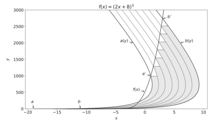
Mathematicians in South Africa have used Cavalieri's principle to calculate areas bounded by curves using Riemann-Stieltjes integrals.[12] The integration strips of Riemann integration are replaced with strips that are non-rectangular in shape. The method is to transform a "Cavaliere region" with a transformation h, or to use g = h–1 as integrator.
For a given function f(x) on an interval [a,b], a "translational function" a(y) must intersect (x, f(x)) exactly once for any shift in the interval. A "Cavaliere region" is then bounded by f(x), a(y), the x-axis, and b(y) := a(y) + (b – a). The area of the region is then
- where a' and b' are the x-values where a(y) and b(y) intersect f(x).

Notes
- Stieltjes (1894), pp. 68–71.
- Hille & Phillips (1974), §3.3.
- Young (1936).
- See Riesz & Sz. Nagy (1990) for details.
- Johnsonbaugh & Pfaffenberger (2010), p. 219.
- Rudin (1964), pp. 121–122.
- Kolmogorov & Fomin (1975), p. 368.
- Introduced by Pollard (1920) and now standard in analysis.
- McShane (1952).
- Hildebrandt (1938) calls it the Pollard–Moore–Stieltjes integral.
- Graves (1946), Chap. XII, §3.
- T. L. Grobler, E. R. Ackermann, A. J. van Zyl & J. C. Olivier Cavaliere integration from Council for Scientific and Industrial Research
References
- Graves, Lawrence (1946). The Theory of Functions of Real Variables. McGraw-Hill.CS1 maint: ref=harv (link) via HathiTrust
- Hildebrandt, T.H. (1938). "Definitions of Stieltjes integrals of the Riemann type". The American Mathematical Monthly. 45 (5): 265–278. ISSN 0002-9890. JSTOR 2302540. MR 1524276.CS1 maint: ref=harv (link)
- Hille, Einar; Phillips, Ralph S. (1974). Functional analysis and semi-groups. Providence, RI: American Mathematical Society. MR 0423094.CS1 maint: ref=harv (link)
- Johnsonbaugh, Richard F.; Pfaffenberger, William Elmer (2010). Foundations of mathematical analysis. Mineola, NY: Dover Publications. ISBN 978-0-486-47766-4.CS1 maint: ref=harv (link)
- Kolmogorov, Andrey; Fomin, Sergei V. (1975) [1970]. Introductory Real Analysis. Translated by Silverman, Richard A. (Revised English ed.). Dover Press. ISBN 0-486-61226-0.CS1 maint: ref=harv (link)
- McShane, E. J. (1952). "Partial orderings & Moore-Smith limit" (PDF). The American Mathematical Monthly. 59: 1–11. doi:10.2307/2307181. JSTOR 2307181. Retrieved 2 November 2010.CS1 maint: ref=harv (link)
- Pollard, Henry (1920). "The Stieltjes integral and its generalizations". The Quarterly Journal of Pure and Applied Mathematics. 19.CS1 maint: ref=harv (link)
- Riesz, F.; Sz. Nagy, B. (1990). Functional Analysis. Dover Publications. ISBN 0-486-66289-6.CS1 maint: ref=harv (link)
- Rudin, Walter (1964). Principles of mathematical analysis (Second ed.). New York, NY: McGraw-Hill.CS1 maint: ref=harv (link)
- Shilov, G. E.; Gurevich, B. L. (1978). Integral, Measure, and Derivative: A unified approach. Translated by Silverman, Richard A. Dover Publications. Bibcode:1966imdu.book.....S. ISBN 0-486-63519-8.
- Stieltjes, Thomas Jan (1894). "Recherches sur les fractions continues". Ann. Fac. Sci. Toulouse. VIII: 1–122. MR 1344720.CS1 maint: ref=harv (link)
- Stroock, Daniel W. (1998). A Concise Introduction to the Theory of Integration (3rd ed.). Birkhauser. ISBN 0-8176-4073-8.
- Young, L.C. (1936). "An inequality of the Hölder type, connected with Stieltjes integration". Acta Mathematica. 67 (1): 251–282. doi:10.1007/bf02401743.CS1 maint: ref=harv (link)