Rankine–Hugoniot conditions

The Rankine–Hugoniot conditions, also referred to as Rankine–Hugoniot jump conditions or Rankine–Hugoniot relations, describe the relationship between the states on both sides of a shock wave or a combustion wave (deflagration or detonation) in a one-dimensional flow in fluids or a one-dimensional deformation in solids. They are named in recognition of the work carried out by Scottish engineer and physicist William John Macquorn Rankine[1] and French engineer Pierre Henri Hugoniot.[2][3]

A schematic diagram of a shock wave situation with the density

\rho

, velocity

u

, and temperature

T

indicated for each region.

In a coordinate system that is moving with the discontinuity, the Rankine–Hugoniot conditions can be expressed as:[4]

{\begin{aligned}\rho _{1}\,u_{1}&=\rho _{2}\,u_{2}\equiv m&&{\text{Conservation of mass}}\\\rho _{1}\,u_{1}^{2}+p_{1}&=\rho _{2}\,u_{2}^{2}+p_{2}&&{\text{Conservation of momentum}}\\h_{1}+{\frac {1}{2}}u_{1}^{2}&=h_{2}+{\frac {1}{2}}u_{2}^{2}&&{\text{Conservation of energy}}\end{aligned}}

where m is the mass flow rate per unit area, ρ₁ and ρ₂ are the mass density of the fluid upstream and downstream of the wave, u₁ and u₂ are the fluid velocity upstream and downstream of the wave, p₁ and p₂ are the pressures in the two regions, and h₁ and h₂ are the specific (with the sense of per unit mass) enthalpies in the two regions. If in addition, the flow is reactive, then the species conservation equations demands that

\omega _{i,1}=\omega _{i,2}=0,\quad i=1,2,3,...N,\qquad {\text{Conservation of species}}

to vanish both upstream and downstream of the discontinuity. Here, $\omega$ is the mass production rate of the ith species of total N species involved in the reaction. Combining conservation of mass and momentum gives us

{\frac {p_{2}-p_{1}}{1/\rho _{2}-1/\rho _{1}}}=-m^{2}

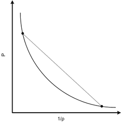
which defines a straight line known as the Rayleigh line, named after Lord Rayleigh, that has a negative slope (since $m^{2}$ is always positive) in the $p-\rho ^{-1}$ plane. Using the Rankine–Hugoniot equations for the conservation of mass and momentum to eliminate u₁ and u₂, the equation for the conservation of energy can be expressed as the Hugoniot equation:

h_{2}-h_{1}={\frac {1}{2}}\,\left({\frac {1}{\rho _{2}}}+{\frac {1}{\rho _{1}}}\right)\,(p_{2}-p_{1}).

The inverse of the density can also be expressed as the specific volume, $v=1/\rho$ . Along with these, one has to specify the relation between the upstream and downstream equation of state

f(p_{1},\rho _{1},T_{1},Y_{i,1})=f(p_{2},\rho _{2},T_{2},Y_{i,2})

where $Y_{i}$ is the mass fraction of the species. Finally, the calorific equation of state $h=h(p,\rho ,Y_{i})$ is assumed to be known, i.e.,

h(p_{1},\rho _{1},Y_{i,1})=h(p_{2},\rho _{2},Y_{i,2}).

Simplified Rankine–Hugoniot relations[5]

The following assumptions are made in order to simplify the Rankine–Hugoniot equations. The mixture is assumed to obey the ideal gas law, so that relation between the downstream and upstream equation of state can be written as

{\frac {p_{2}}{\rho _{2}T_{2}}}={\frac {p_{1}}{\rho _{1}T_{1}}}={\frac {R}{\overline {W}}}

where $R$ is the universal gas constant and the mean molecular weight ${\overline {W}}$ is assumed to be constant (otherwise, ${\overline {W}}$ would depend on the mass fraction of the all species). If one assumes that the specific heat at constant pressure $c_{p}$ is also constant across the wave, the change in enthalpies (calorific equation of state) can be simply written as

h_{2}-h_{1}=-q+c_{p}(T_{2}-T_{1})

where the first term in the above expression represents the amount of heat released per unit mass of the upstream mixture by the wave and the second term represents the sensible heating. Eliminating temperature using the equation of state and substituting the above expression for the change in enthalpies into the Hugoniot equation, one obtains a Hugoniot equation expressed only in terms of pressure and densities,

\left({\frac {\gamma }{\gamma -1}}\right)\left({\frac {p_{2}}{\rho _{2}}}-{\frac {p_{1}}{\rho _{1}}}\right)-{\frac {1}{2}}\left({\frac {1}{\rho _{2}}}+{\frac {1}{\rho _{1}}}\right)(p_{2}-p_{1})=q,

where $\gamma$ is the specific heat ratio. Hugoniot curve without heat release ( $q=0$ ) is often called as Shock Hugoniot. Along with the Rayleigh line equation, the above equation completely determines the state of the system. These two equations can be written compactly by introducing the following non-dimensional scales,

{\tilde {p}}={\frac {p_{2}}{p_{1}}},\quad {\tilde {v}}={\frac {\rho _{1}}{\rho _{2}}},\quad \alpha ={\frac {q\rho _{1}}{p_{1}}},\quad \mu ={\frac {m^{2}}{p_{1}\rho _{1}}}.

The Rayleigh line equation and the Hugoniot equation then simplifies to

{\begin{aligned}{\frac {{\tilde {p}}-1}{{\tilde {v}}-1}}&=-\mu \\{\tilde {p}}&={\frac {[2\alpha +(\gamma +1)/(\gamma -1)]-{\tilde {v}}}{[(\gamma +1)/(\gamma -1)]{\tilde {v}}-1}}.\end{aligned}}

Given the upstream conditions, the intersection of above two equations in the ${\tilde {p}}-{\tilde {v}}$ plane determine the downstream conditions. If no heat release occurs, for example, shock waves without chemical reaction, then $\alpha =0$ . The Hugoniot curves asymptote to the lines ${\tilde {v}}=(\gamma -1)/(\gamma +1)$ and ${\tilde {p}}=-(\gamma -1)/(\gamma +1)$ , i.e., the pressure jump across the wave can take any values between $0\leq {\tilde {p}}<\infty$ , but the specific volume ratio is restricted to the interval $(\gamma -1)/(\gamma +1)\leq {\tilde {v}}\leq 2\alpha +(\gamma +1)/(\gamma -1)$ (the upper bound is derived for the case ${\tilde {p}}\rightarrow 0$ because pressure cannot take negative values). The Chapman–Jouguet condition is where Rayleigh line is tangent to the Hugoniot curve.

If $\gamma =1.4$ (diatomic gas without the vibrational mode excitation), the interval is $1/6\leq {\tilde {v}}\leq 2\alpha +6$ , in other words, the shock wave can increase the density at most by a factor of 6. For monoatomic gas, $\gamma =5/3$ , therefore the density ratio is limited by the interval $1/4\leq {\tilde {v}}\leq 2\alpha +4$ . For diatomic gases with vibrational mode excited, we have $\gamma =9/7$ leading to the interval $1/8\leq {\tilde {v}}\leq 2\alpha +8$ . In reality, the specific heat ratio is not constant in the shock wave due to molecular dissociation and ionization, but even in these cases, density ratio in general do not exceed the factor $11-13$ .[6]

Derivation from Euler equations

Consider gas in a one-dimensional container (e.g., a long thin tube). Assume that the fluid is inviscid (i.e., it shows no viscosity effects as for example friction with the tube walls). Furthermore, assume that there is no heat transfer by conduction or radiation and that gravitational acceleration can be neglected. Such a system can be described by the following system of conservation laws, known as the 1D Euler equations, that in conservation form is:

(\;1)\quad \quad {\frac {\partial \rho }{\partial t}}\;\;=-{\frac {\partial }{\partial x}}\left(\rho u\right)

(\;2)\quad \quad {\frac {\partial }{\partial t}}(\rho u)\,=-{\frac {\partial }{\partial x}}\left(\rho u^{2}+p\right)

(\;3)\quad \quad {\frac {\partial }{\partial t}}\left(E^{t}\right)=-{\frac {\partial }{\partial x}}\left[u\left(E^{t}+p\right)\right],

where

\rho ,\,

fluid mass density,

u,\,

fluid velocity,

e,\,

specific internal energy of the fluid,

p,\,

fluid pressure, and

E^{t}=\rho e+\rho {\frac {1}{2}}u^{2},\,

is the total energy density of the fluid, [J/m³], while e is its specific internal energy

Assume further that the gas is calorically ideal and that therefore a polytropic equation-of-state of the simple form

(\;4)\quad \quad p=\left(\gamma -1\right)\rho e,

is valid, where $\gamma$ is the constant ratio of specific heats $c_{p}/c_{v}$ . This quantity also appears as the polytropic exponent of the polytropic process described by

(\;5)\quad \quad {\frac {p}{\rho ^{\gamma }}}={\text{constant}}.

For an extensive list of compressible flow equations, etc., refer to NACA Report 1135 (1953).[7]

Note: For a calorically ideal gas $\gamma \,$ is a constant and for a thermally ideal gas $\gamma \,$ is a function of temperature. In the latter case, the dependence of pressure on mass density and internal energy might differ from that given by equation (4).

The jump condition

Before proceeding further it is necessary to introduce the concept of a jump condition – a condition that holds at a discontinuity or abrupt change.

Consider a 1D situation where there is a jump in the scalar conserved physical quantity $w$ , which is governed by integral conservation law

(\;6)\quad \quad {\frac {d}{dt}}\int _{x_{1}}^{x_{2}}w\,dx=-\left.f\left(w\right)\right|_{x_{1}}^{x_{2}}

for any $x_{1}$ , $x_{2}$ , $x_{1}<x_{2}$ , and, therefore, by partial differential equation

(\;6')\quad \quad {\frac {\partial w}{\partial t}}+{\frac {\partial }{\partial x}}f\left(w\right)=0

for smooth solutions.[8]

Let the solution exhibit a jump (or shock) at $x=x_{s}(t)$ , where $x_{1}<x_{s}(t)$ and $x_{s}(t)<x_{2}$ , then

(\;7)\quad \quad {\frac {d}{dt}}\left[\left(\int _{x_{1}}^{x_{s}(t)}w\,dx+\int _{x_{s}(t)}^{x_{2}}w\,dx\right)\right]=-\int _{x_{1}}^{x_{2}}{\frac {\partial }{\partial x}}f\left(w\right)\,dx

(\;8)\quad \quad \therefore w_{1}{\frac {dx_{s}}{dt}}-w_{2}{\frac {dx_{s}}{dt}}+\int _{x_{1}}^{x_{s}(t)}w_{t}\,dx+\int _{x_{s}(t)}^{x_{2}}w_{t}\,dx=-\left.f\left(w\right)\right|_{x_{1}}^{x_{2}}

The subscripts 1 and 2 indicate conditions just upstream and just downstream of the jump respectively, i.e. $w_{1}=\lim _{\epsilon \rightarrow 0^{+}}w\left(x_{s}-\epsilon \right)$ and $w_{2}=\lim _{\epsilon \rightarrow 0^{+}}w\left(x_{s}+\epsilon \right)$ .

Note, to arrive at equation (8) we have used the fact that $dx_{1}/dt=0$ and $dx_{2}/dt=0$ .

Now, let $x_{1}\rightarrow x_{s}(t)-\epsilon$ and $x_{2}\rightarrow x_{s}(t)+\epsilon$ , when we have $\int _{x_{1}}^{x_{s}(t)-\epsilon }w_{t}\,dx\rightarrow 0$ and $\int _{x_{s}(t)+\epsilon }^{x_{2}}w_{t}\,dx\rightarrow 0$ , and in the limit

(\;9)\quad \quad u_{s}\left(w_{1}-w_{2}\right)=f\left(w_{1}\right)-f\left(w_{2}\right),

where we have defined $u_{s}=dx_{s}(t)/dt\,$ (the system characteristic or shock speed), which by simple division is given by

(10)\quad \quad u_{s}={\frac {f\left(w_{1}\right)-f\left(w_{2}\right)}{w_{1}-w_{2}}}.

Equation (9) represents the jump condition for conservation law (6). A shock situation arises in a system where its characteristics intersect, and under these conditions a requirement for a unique single-valued solution is that the solution should satisfy the admissibility condition or entropy condition. For physically real applications this means that the solution should satisfy the Lax entropy condition

(11)\quad \quad f^{\prime }\left(w_{1}\right)>u_{s}>f^{\prime }\left(w_{2}\right),

where $f^{\prime }\left(w_{1}\right)$ and $f^{\prime }\left(w_{2}\right)$ represent characteristic speeds at upstream and downstream conditions respectively.

Shock condition

In the case of the hyperbolic conservation law (6), we have seen that the shock speed can be obtained by simple division. However, for the 1D Euler equations ( 1), ( 2) and ( 3), we have the vector state variable ${\begin{bmatrix}\rho &\rho u&E\end{bmatrix}}^{\mathsf {T}}$ and the jump conditions become

(12)\quad \quad \quad \quad \;u_{s}\left(\rho _{2}-\rho _{1}\right)=\rho _{2}u_{2}-\rho _{1}u_{1}

(13)\quad \quad \;u_{s}\left(\rho _{2}u_{2}-\rho _{1}u_{1}\right)=\left(\rho _{2}u_{2}^{2}+p_{2}\right)-\left(\rho _{1}u_{1}^{2}+p_{1}\right)

(14)\quad \quad u_{s}\left(E_{2}-E_{1}\right)=\left[\rho _{2}u_{2}\left(e_{2}+{\frac {1}{2}}u_{2}^{2}+{\frac {p_{2}}{\rho _{2}}}\right)\right]-\left[\rho _{1}u_{1}\left(e_{1}+{\frac {1}{2}}u_{1}^{2}+{\frac {p_{1}}{\rho _{1}}}\right)\right].

Equations (12), (13) and (14) are known as the Rankine–Hugoniot conditions for the Euler equations and are derived by enforcing the conservation laws in integral form over a control volume that includes the shock. For this situation $u_{s}$ cannot be obtained by simple division. However, it can be shown by transforming the problem to a moving co-ordinate system (setting $u_{s}':=u_{s}-u_{1}$ , $u'_{1}:=0$ , $u'_{2}:=u_{2}-u_{1}$ to remove $u_{1}$ ) and some algebraic manipulation (involving the elimination of $u'_{2}$ from the transformed equation (13) using the transformed equation (12)), that the shock speed is given by

(15)\quad \quad u_{s}=u_{1}+c_{1}{\sqrt {1+{\frac {\gamma +1}{2\gamma }}\left({\frac {p_{2}}{p_{1}}}-1\right)}},

where $c_{1}={\sqrt {\gamma p_{1}/\rho _{1}}}$ is the speed of sound in the fluid at upstream conditions.[9][10][11][12][13][14]

Shock Hugoniot and Rayleigh line in solids

Shock Hugoniot and Rayleigh line in the p-v plane. The curve represents a plot of equation (24) with p₁, v₁, c₀, and s known. If p₁ = 0, the curve will intersect the specific volume axis at the point v₁.

Hugoniot elastic limit in the p-v plane for a shock in an elastic-plastic material.

For shocks in solids, a closed form expression such as equation (15) cannot be derived from first principles. Instead, experimental observations[15] indicate that a linear relation[16] can be used instead (called the shock Hugoniot in the u_s-u_p plane) that has the form

u_{s}=c_{0}+s\,u_{p}=c_{0}+s\,u_{2}

where c₀ is the bulk speed of sound in the material (in uniaxial compression), s is a parameter (the slope of the shock Hugoniot) obtained from fits to experimental data, and u_p = u₂ is the particle velocity inside the compressed region behind the shock front.

The above relation, when combined with the Hugoniot equations for the conservation of mass and momentum, can be used to determine the shock Hugoniot in the p-v plane, where v is the specific volume (per unit mass):[17]

p_{2}-p_{1}={\frac {c_{0}^{2}\,\rho _{1}\,\rho _{2}\,\left(\rho _{2}-\rho _{1}\right)}{\left[\rho _{2}-s\left(\rho _{2}-\rho _{1}\right)\right]^{2}}}={\frac {c_{0}^{2}\,\left(v_{1}-v_{2}\right)}{\left[v_{1}-s\left(v_{1}-v_{2}\right)\right]^{2}}}\,.

Alternative equations of state, such as the Mie–Grüneisen equation of state may also be used instead of the above equation.

The shock Hugoniot describes the locus of all possible thermodynamic states a material can exist in behind a shock, projected onto a two dimensional state-state plane. It is therefore a set of equilibrium states and does not specifically represent the path through which a material undergoes transformation.

Weak shocks are isentropic and that the isentrope represents the path through which the material is loaded from the initial to final states by a compression wave with converging characteristics. In the case of weak shocks, the Hugoniot will therefore fall directly on the isentrope and can be used directly as the equivalent path. In the case of a strong shock we can no longer make that simplification directly. However, for engineering calculations, it is deemed that the isentrope is close enough to the Hugoniot that the same assumption can be made.

If the Hugoniot is approximately the loading path between states for an "equivalent" compression wave, then the jump conditions for the shock loading path can be determined by drawing a straight line between the initial and final states. This line is called the Rayleigh line and has the following equation:

p_{2}-p_{1}=u_{s}^{2}\left(\rho _{1}-{\frac {\rho _{1}^{2}}{\rho _{2}}}\right)\,

Hugoniot elastic limit

Most solid materials undergo plastic deformations when subjected to strong shocks. The point on the shock Hugoniot at which a material transitions from a purely elastic state to an elastic-plastic state is called the Hugoniot elastic limit (HEL) and the pressure at which this transition takes place is denoted p_HEL. Values of p_HEL can range from 0.2 GPa to 20 GPa. Above the HEL, the material loses much of its shear strength and starts behaving like a fluid.

References

Rankine, W. J. M. (1870). "On the thermodynamic theory of waves of finite longitudinal disturbances". Philosophical Transactions of the Royal Society of London. 160: 277–288. doi:10.1098/rstl.1870.0015.
Hugoniot, H. (1887). "Mémoire sur la propagation des mouvements dans les corps et spécialement dans les gaz parfaits (première partie) [Memoir on the propagation of movements in bodies, especially perfect gases (first part)]". Journal de l'École Polytechnique (in French). 57: 3–97. See also: Hugoniot, H. (1889) "Mémoire sur la propagation des mouvements dans les corps et spécialement dans les gaz parfaits (deuxième partie)" [Memoir on the propagation of movements in bodies, especially perfect gases (second part)], Journal de l'École Polytechnique, vol. 58, pages 1–125.
Salas, M. D. (2006). "The Curious Events Leading to the Theory of Shock Waves, Invited lecture, 17th Shock Interaction Symposium, Rome, 4–8 September" (PDF).
Williams, F. A. (2018). Combustion theory. CRC Press.
Williams, F. A. (2018). Combustion theory. CRC Press.
Zel’Dovich, Y. B., & Raizer, Y. P. (2012). Physics of shock waves and high-temperature hydrodynamic phenomena. Courier Corporation.
Ames Research Staff (1953), "Equations, Tables and Charts for Compressible Flow" (PDF), Report 1135 of the National Advisory Committee for Aeronautics
Note that the integral conservation law $\scriptstyle (6)$ could not, in general, be obtained from differential equation $\scriptstyle (6')$ by integraition over $\scriptstyle [x_{1};x_{2}]$ because $\scriptstyle (6')$ holds for smooth solutions only.
Liepmann, H. W., & Roshko, A. (1957). Elements of gasdynamics. Courier Corporation.
Landau, L. D. (1959). EM Lifshitz, Fluid Mechanics. Course of Theoretical Physics, 6.
Shapiro, A. H. (1953). The dynamics and thermodynamics of compressible fluid flow. John Wiley & Sons.
Anderson, J. D. (1990). Modern compressible flow: with historical perspective (Vol. 12). New York: McGraw-Hill.
Whitham, G. B. (1999). Linear and Nonlinear Waves. Wiley. ISBN 978-0-471-94090-6.
Courant, R., & Friedrichs, K. O. (1999). Supersonic flow and shock waves (Vol. 21). Springer Science & Business Media.
Ahrens, T.J. (1993), "Equation of state" (PDF), High Pressure Shock Compression of Solids, Eds. J. R. Asay and M. Shahinpoor, Springer-Verlag, New York: 75–113, doi:10.1007/978-1-4612-0911-9_4, ISBN 978-1-4612-6943-4
Though a linear relation is widely assumed to hold, experimental data suggest that almost 80% of tested materials do not satisfy this widely accepted linear behavior. See Kerley, G. I, 2006, "The Linear US-uP Relation in Shock-Wave Physics", arXiv:1306.6916; for details.
Poirier, J-P. (2008) "Introduction to the Physics of the Earth's Interior", Cambridge University Press.

This article is issued from Wikipedia. The text is licensed under Creative Commons - Attribution - Sharealike. Additional terms may apply for the media files.

[[Ran-70]-1] Rankine, W. J. M. (1870). "On the thermodynamic theory of waves of finite longitudinal disturbances". Philosophical Transactions of the Royal Society of London. 160: 277–288. doi:10.1098/rstl.1870.0015.

[[Hug-87]-2] Hugoniot, H. (1887). "Mémoire sur la propagation des mouvements dans les corps et spécialement dans les gaz parfaits (première partie) [Memoir on the propagation of movements in bodies, especially perfect gases (first part)]". Journal de l'École Polytechnique (in French). 57: 3–97. See also: Hugoniot, H. (1889) "Mémoire sur la propagation des mouvements dans les corps et spécialement dans les gaz parfaits (deuxième partie)" [Memoir on the propagation of movements in bodies, especially perfect gases (second part)], Journal de l'École Polytechnique, vol. 58, pages 1–125.

[[Sal-06]-3] Salas, M. D. (2006). "The Curious Events Leading to the Theory of Shock Waves, Invited lecture, 17th Shock Interaction Symposium, Rome, 4–8 September" (PDF).

[4] Williams, F. A. (2018). Combustion theory. CRC Press.

[5] Williams, F. A. (2018). Combustion theory. CRC Press.

[6] Zel’Dovich, Y. B., & Raizer, Y. P. (2012). Physics of shock waves and high-temperature hydrodynamic phenomena. Courier Corporation.

[[Ame-53]-7] Ames Research Staff (1953), "Equations, Tables and Charts for Compressible Flow" (PDF), Report 1135 of the National Advisory Committee for Aeronautics

[8] Note that the integral conservation law $\scriptstyle (6)$ could not, in general, be obtained from differential equation $\scriptstyle (6')$ by integraition over $\scriptstyle [x_{1};x_{2}]$ because $\scriptstyle (6')$ holds for smooth solutions only.

[9] Liepmann, H. W., & Roshko, A. (1957). Elements of gasdynamics. Courier Corporation.

[10] Landau, L. D. (1959). EM Lifshitz, Fluid Mechanics. Course of Theoretical Physics, 6.

[11] Shapiro, A. H. (1953). The dynamics and thermodynamics of compressible fluid flow. John Wiley & Sons.

[12] Anderson, J. D. (1990). Modern compressible flow: with historical perspective (Vol. 12). New York: McGraw-Hill.

[[Whi-99]-13] Whitham, G. B. (1999). Linear and Nonlinear Waves. Wiley. ISBN 978-0-471-94090-6.

[14] Courant, R., & Friedrichs, K. O. (1999). Supersonic flow and shock waves (Vol. 21). Springer Science & Business Media.

[15] Ahrens, T.J. (1993), "Equation of state" (PDF), High Pressure Shock Compression of Solids, Eds. J. R. Asay and M. Shahinpoor, Springer-Verlag, New York: 75–113, doi:10.1007/978-1-4612-0911-9_4, ISBN 978-1-4612-6943-4

[Kerley-16] Though a linear relation is widely assumed to hold, experimental data suggest that almost 80% of tested materials do not satisfy this widely accepted linear behavior. See Kerley, G. I, 2006, "The Linear US-uP Relation in Shock-Wave Physics", arXiv:1306.6916; for details.

[17] Poirier, J-P. (2008) "Introduction to the Physics of the Earth's Interior", Cambridge University Press.