Q-function
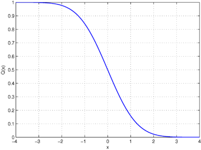
In statistics, the Q-function is the tail distribution function of the standard normal distribution.[1][2] In other words, is the probability that a normal (Gaussian) random variable will obtain a value larger than standard deviations. Equivalently, is the probability that a standard normal random variable takes a value larger than .


If is a Gaussian random variable with mean and variance , then is standard normal and


where .

Other definitions of the Q-function, all of which are simple transformations of the normal cumulative distribution function, are also used occasionally.[3]
Because of its relation to the cumulative distribution function of the normal distribution, the Q-function can also be expressed in terms of the error function, which is an important function in applied mathematics and physics.
Definition and basic properties
Formally, the Q-function is defined as

Thus,

where is the cumulative distribution function of the standard normal Gaussian distribution.

The Q-function can be expressed in terms of the error function, or the complementary error function, as[2]

An alternative form of the Q-function known as Craig's formula, after its discoverer, is expressed as:[4]

This expression is valid only for positive values of x, but it can be used in conjunction with Q(x) = 1 − Q(−x) to obtain Q(x) for negative values. This form is advantageous in that the range of integration is fixed and finite.
Craig's formula was later extended by Behnad (2020)[5] for the Q-function of the sum of two non-negative variables, as follows:

Bounds and approximations
- The Q-function is not an elementary function. However, the bounds, where is the density function of the standard normal distribution,[6]


- become increasingly tight for large x, and are often useful.
- Using the substitution v =u2/2, the upper bound is derived as follows:

- Similarly, using and the quotient rule,


- Solving for Q(x) provides the lower bound.
- The geometric mean of the upper and lower bound gives a suitable approximation for Q(x):

- Tighter bounds and approximations of the Q(x) can also be obtained by optimizing the following expression [6]

- For , the best upper bound is given by and with maximum absolute relative error of 0.44%. Likewise, the best approximation is given by and with maximum absolute relative error of 0.27%. Finally, the best lower bound is given by and with maximum absolute relative error of 1.17%.


- The Chernoff bound of the Q-function is

- Improved exponential bounds and a pure exponential approximation are [7]


- Another approximation of for is given by Karagiannidis & Lioumpas (2007)[8] who showed for the appropriate choice of parameters that


- The absolute error between and over the range is minimized by evaluating


- Using and numerically integrating, they found the minimum error occurred when which gave a good approximation for


- Substituting these values and using the relationship between and from above gives

- A tighter and more tractable approximation of for positive arguments is given by López-Benítez & Casadevall (2011)[9] based on a second-order exponential function:

- The fitting coefficients can be optimized over any desired range of arguments in order to minimize the sum of square errors (, , for ) or minimize the maximum absolute error (, , for ). This approximation offers some benefits such as a good trade-off between accuracy and analytical tractability (for example, the extension to any arbitrary power of is trivial and does not alter the algebraic form of the approximation).


Inverse Q
The inverse Q-function can be related to the inverse error functions:

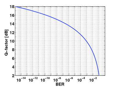
The function finds application in digital communications. It is usually expressed in dB and generally called Q-factor:


where y is the bit-error rate (BER) of the digitally modulated signal under analysis. For instance, for QPSK in additive white Gaussian noise, the Q-factor defined above coincides with the value in dB of the signal to noise ratio that yields a bit error rate equal to y.
Values
The Q-function is well tabulated and can be computed directly in most of the mathematical software packages such as R and those available in Python, MATLAB and Mathematica. Some values of the Q-function are given below for reference.
|
|
|
|
Generalization to high dimensions
The Q-function can be generalized to higher dimensions:[10]

where follows the multivariate normal distribution with covariance and the threshold is of the form for some positive vector and positive constant . As in the one dimensional case, there is no simple analytical formula for the Q-function. Nevertheless, the Q-function can be approximated arbitrarily well as becomes larger and larger.[11][12]


References
- The Q-function, from cnx.org
- Basic properties of the Q-function Archived March 25, 2009, at the Wayback Machine
- Normal Distribution Function - from Wolfram MathWorld
- Craig, J.W. (1991). "A new, simple and exact result for calculating the probability of error for two-dimensional signal constellations" (PDF). MILCOM 91 - Conference record. pp. 571–575. doi:10.1109/MILCOM.1991.258319. ISBN 0-87942-691-8.
- Behnad, Aydin (2020). "A Novel Extension to Craig's Q-Function Formula and Its Application in Dual-Branch EGC Performance Analysis". IEEE Transactions on Communications (Early Access). doi:10.1109/TCOMM.2020.2986209.
- Borjesson, P.; Sundberg, C.-E. (1979). "Simple Approximations of the Error Function Q(x) for Communications Applications". IEEE Transactions on Communications. 27 (3): 639–643. doi:10.1109/TCOM.1979.1094433.
- Chiani, M.; Dardari, D.; Simon, M.K. (2003). "New exponential bounds and approximations for the computation of error probability in fading channels" (PDF). IEEE Transactions on Wireless Communications. 24 (5): 840–845. doi:10.1109/TWC.2003.814350.
- Karagiannidis, George; Lioumpas, Athanasios (2007). "An Improved Approximation for the Gaussian Q-Function" (PDF). IEEE Communications Letters. 11 (8): 644–646. doi:10.1109/LCOMM.2007.070470.
- Lopez-Benitez, Miguel; Casadevall, Fernando (2011). "Versatile, Accurate, and Analytically Tractable Approximation for the Gaussian Q-Function" (PDF). IEEE Transactions on Communications. 59 (4): 917–922. doi:10.1109/TCOMM.2011.012711.100105.
- Savage, I. R. (1962). "Mills ratio for multivariate normal distributions". Journal of Research of the National Bureau of Standards Section B. 66: 93–96. Zbl 0105.12601.
- Botev, Z. I. (2016). "The normal law under linear restrictions: simulation and estimation via minimax tilting". Journal of the Royal Statistical Society, Series B. 79: 125–148. arXiv:1603.04166. Bibcode:2016arXiv160304166B. doi:10.1111/rssb.12162.
- Botev, Z. I.; Mackinlay, D.; Chen, Y.-L. (2017). "Logarithmically efficient estimation of the tail of the multivariate normal distribution". 2017 Winter Simulation Conference (WSC). IEEE. pp. 1903–191. doi:10.1109/WSC.2017.8247926. ISBN 978-1-5386-3428-8.