Pathfinding
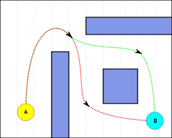
Pathfinding or pathing is the plotting, by a computer application, of the shortest route between two points. It is a more practical variant on solving mazes. This field of research is based heavily on Dijkstra's algorithm for finding the shortest path on a weighted graph.
| Graph and tree search algorithms |
|---|
| Listings |
|
| Related topics |
Pathfinding is closely related to the shortest path problem, within graph theory, which examines how to identify the path that best meets some criteria (shortest, cheapest, fastest, etc) between two points in a large network.
Algorithms
At its core, a pathfinding method searches a graph by starting at one vertex and exploring adjacent nodes until the destination node is reached, generally with the intent of finding the cheapest route. Although graph searching methods such as a breadth-first search would find a route if given enough time, other methods, which "explore" the graph, would tend to reach the destination sooner. An analogy would be a person walking across a room; rather than examining every possible route in advance, the person would generally walk in the direction of the destination and only deviate from the path to avoid an obstruction, and make deviations as minor as possible.
Two primary problems of pathfinding are (1) to find a path between two nodes in a graph; and (2) the shortest path problem—to find the optimal shortest path. Basic algorithms such as breadth-first and depth-first search address the first problem by exhausting all possibilities; starting from the given node, they iterate over all potential paths until they reach the destination node. These algorithms run in , or linear time, where V is the number of vertices, and E is the number of edges between vertices.

The more complicated problem is finding the optimal path. The exhaustive approach in this case is known as the Bellman–Ford algorithm, which yields a time complexity of , or quadratic time. However, it is not necessary to examine all possible paths to find the optimal one. Algorithms such as A* and Dijkstra's algorithm strategically eliminate paths, either through heuristics or through dynamic programming. By eliminating impossible paths, these algorithms can achieve time complexities as low as .[1]


The above algorithms are among the best general algorithms which operate on a graph without preprocessing. However, in practical travel-routing systems, even better time complexities can be attained by algorithms which can pre-process the graph to attain better performance.[2] One such algorithm is contraction hierarchies.
Dijkstra's algorithm
A common example of a graph-based pathfinding algorithm is Dijkstra's algorithm. This algorithm begins with a start node and an "open set" of candidate nodes. At each step, the node in the open set with the lowest distance from the start is examined. The node is marked "closed", and all nodes adjacent to it are added to the open set if they have not already been examined. This process repeats until a path to the destination has been found. Since the lowest distance nodes are examined first, the first time the destination is found, the path to it will be the shortest path.[3]
Dijkstra's algorithm fails if there is a negative edge weight. In the hypothetical situation where Nodes A, B, and C form a connected undirected graph with edges AB = 3, AC = 4, and BC = −2, the optimal path from A to C costs 1, and the optimal path from A to B costs 2. Dijkstra's Algorithm starting from A will first examine B, as that is the closest. It will assign a cost of 3 to it, and mark it closed, meaning that its cost will never be reevaluated. Therefore, Dijkstra's cannot evaluate negative edge weights. However, since for many practical purposes there will never be a negative edgeweight, Dijkstra's algorithm is largely suitable for the purpose of pathfinding.
A* algorithm
A* is a variant of Dijkstra's algorithm commonly used in games. A* assigns a weight to each open node equal to the weight of the edge to that node plus the approximate distance between that node and the finish. This approximate distance is found by the heuristic, and represents a minimum possible distance between that node and the end. This allows it to eliminate longer paths once an initial path is found. If there is a path of length x between the start and finish, and the minimum distance between a node and the finish is greater than x, that node need not be examined.[4]
A* uses this heuristic to improve on the behavior relative to Dijkstra's algorithm. When the heuristic evaluates to zero, A* is equivalent to Dijkstra's algorithm. As the heuristic estimate increases and gets closer to the true distance, A* continues to find optimal paths, but runs faster (by virtue of examining fewer nodes). When the value of the heuristic is exactly the true distance, A* examines the fewest nodes. (However, it is generally impractical to write a heuristic function that always computes the true distance, as the same comparison result can often be reached using simpler calculations – for example, using Manhattan distance over Euclidean distance in two-dimensional space.) As the value of the heuristic increases, A* examines fewer nodes but no longer guarantees an optimal path. In many applications (such as video games) this is acceptable and even desirable, in order to keep the algorithm running quickly.
Sample algorithm
This is a fairly simple and easy-to-understand pathfinding algorithm for tile-based maps. To start off, you have a map, a start coordinate and a destination coordinate. The map will look like this, X being walls, S being the start, O being the finish and _ being open spaces, the numbers along the top and right edges are the column and row numbers:
  1 2 3 4 5 6 7 8
X X X X X X X X X X
X _ _ _ X X _ X _ X 1
X _ X _ _ X _ _ _ X 2
X S X X _ _ _ X _ X 3
X _ X _ _ X _ _ _ X 4
X _ _ _ X X _ X _ X 5
X _ X _ _ X _ X _ X 6
X _ X X _ _ _ X _ X 7
X _ _ O _ X _ _ _ X 8
X X X X X X X X X X
First, create a list of coordinates, which we will use as a queue. The queue will be initialized with one coordinate, the end coordinate. Each coordinate will also have a counter variable attached (the purpose of this will soon become evident). Thus, the queue starts off as ((3,8,0)).
Then, go through every element in the queue, including elements added to the end over the course of the algorithm, and to each element, do the following:
- Create a list of the four adjacent cells, with a counter variable of the current element's counter variable + 1 (in our example, the four cells are ((2,8,1),(3,7,1),(4,8,1),(3,9,1)))
- Check all cells in each list for the following two conditions:
- If the cell is a wall, remove it from the list
- If there is an element in the main list with the same coordinate and a less than or equal counter, remove it from the cells list
- Add all remaining cells in the list to the end of the main list
- Go to the next item in the list
Thus, after turn 1, the list of elements is this: ((3,8,0),(2,8,1),(4,8,1))
- After 2 turns: ((3,8,0),(2,8,1),(4,8,1),(1,8,2),(4,7,2))
- After 3 turns: (...(1,7,3),(4,6,3),(5,7,3))
- After 4 turns: (...(1,6,4),(3,6,4),(6,7,4))
- After 5 turns: (...(1,5,5),(3,5,5),(6,6,5),(6,8,5))
- After 6 turns: (...(1,4,6),(2,5,6),(3,4,6),(6,5,6),(7,8,6))
- After 7 turns: (...(1,3,7)) – problem solved, end this stage of the algorithm – note that if you have multiple units chasing the same target (as in many games – the finish to start approach of the algorithm is intended to make this easier), you can continue until the entire map is taken up, all units are reached or a set counter limit is reached
Now, map the counters onto the map, getting this:
  1 2 3 4 5 6 7 8
X X X X X X X X X X
X _ _ _ X X _ X _ X 1
X _ X _ _ X _ _ _ X 2
X S X X _ _ _ X _ X 3
X 6 X 6 _ X _ _ _ X 4
X 5 6 5 X X 6 X _ X 5
X 4 X 4 3 X 5 X _ X 6
X 3 X X 2 3 4 X _ X 7
X 2 1 0 1 X 5 6 _ X 8
X X X X X X X X X X
Now, start at S (7) and go to the nearby cell with the lowest number (unchecked cells cannot be moved to). The path traced is (1,3,7) -> (1,4,6) -> (1,5,5) -> (1,6,4) -> (1,7,3) -> (1,8,2) -> (2,8,1) -> (3,8,0). In the event that two numbers are equally low (for example, if S was at (2,5)), pick a random direction – the lengths are the same. The algorithm is now complete.
In video games
Chris Crawford in 1982 described how he "expended a great deal of time" trying to solve a problem with pathfinding in Tanktics, in which computer tanks became trapped on land within U-shaped lakes. "After much wasted effort I discovered a better solution: delete U-shaped lakes from the map", he said.[5]
Hierarchical path finding
The idea was first described by the video game industry, which had a need for planning in large maps with a low amount of CPU time. The concept of using abstraction and heuristics is older and was first mentioned under the name ABSTRIPS (Abstraction-Based STRIPS)[6] which was used to efficiently search the state spaces of logic games.[7] A similar technique are navigation meshes (navmesh), which are used for geometrical planning in games and multimodal transportation planning which is utilized in travelling salesman problems with more than one transport vehicle.
A map is separated into clusters. On the high-level layer, the path between the clusters is planned. After the plan was found, a second path is planned within a cluster on the lower level.[8] That means, the planning is done in two steps which is a guided local search in the original space. The advantage is, that the number of nodes is smaller and the algorithm performs very well. The disadvantage is, that a hierarchical pathplanner is difficult to implement.[9]
Example
A map has a size of 3000x2000 pixels. Planning a path on a pixel base would take very long. Even an efficient algorithm will need to compute many possible graphs. The reason is, that such a map would contain 6 million pixels overall and the possibilities to explore the geometrical space are endless. The first step for a hierarchical path planner is to divide the map into smaller sub-maps. Each cluster has a size of 300x200 pixel. The number of clusters overall is 10x10=100. In the newly created graph the amount of nodes is small, it is possible to navigate between the 100 clusters, but not within the detailed map. If a valid path was found in the high-level-graph the next step is to plan the path within each cluster. The submap has 300x200 pixel which can be handled by a normal A* pathplanner easily.
Algorithms used in pathfinding
- A* search algorithm
- Dijkstra's algorithm, a special case of the A* search algorithm
- D* a family of incremental heuristic search algorithms for problems in which constraints vary over time or are not completely known when the agent first plans its path
- Any-angle path planning algorithms, a family of algorithms for planning paths that are not restricted to move along the edges in the search graph, designed to be able to take on any angle and thus find shorter and straighter paths
Multi-agent Pathfinding
Multi-agent pathfinding is to find the paths for multiple agents from their current locations to their target locations without colliding with each other, while at the same time optimizing a cost function, such as the sum of the path lengths of all agents. It is a generalization of pathfinding. Many multi-agent pathfinding algorithms are generalized from A*, or based on reduction to other well studied problems such as integer linear programming.[10] However, such algorithms are typically incomplete; in other words, not proven to produce a solution within polynomial time. A different category of algorithms sacrifice optimality for performance by either making use of known navigation patterns (such as traffic flow) or the topology of the problem space.[11]
See also
References
- "7.2.1 Single Source Shortest Paths Problem: Dijkstra's Algorithm". Archived from the original on 2016-03-04. Retrieved 2012-05-18.
- Delling, D.; Sanders, P.; Schultes, D.; Wagner, D. (2009). "Engineering route planning algorithms". Algorithmics of Large and Complex Networks: Design, Analysis, and Simulation. Lecture Notes in Computer Science. 5515. Springer. pp. 117–139. CiteSeerX 10.1.1.164.8916. doi:10.1007/978-3-642-02094-0_7. ISBN 978-3-642-02093-3.
- "5.7.1 Dijkstra Algorithm".
- "Introduction to A* Pathfinding".
- Crawford, Chris (December 1982). "Design Techniques and Ideas for Computer Games". BYTE. p. 96. Retrieved 19 October 2013.
- Sacerdoti, Earl D (1974). "Planning in a hierarchy of abstraction spaces" (PDF). Artificial Intelligence. 5 (2): 115–135. doi:10.1016/0004-3702(74)90026-5.
- Holte, Robert C and Perez, MB and Zimmer, RM and MacDonald, AJ (1995). Hierarchical a*. Symposium on Abstraction, Reformulation, and Approximation.CS1 maint: multiple names: authors list (link)
- Pelechano, Nuria and Fuentes, Carlos (2016). "Hierarchical path-finding for Navigation Meshes (HNA⁎)" (PDF). Computers&Graphics. 59: 68–78. doi:10.1016/j.cag.2016.05.023. hdl:2117/98738.CS1 maint: multiple names: authors list (link)
- Botea, Adi and Muller, Martin and Schaeffer, Jonathan (2004). "Near optimal hierarchical path-finding". Journal of Game Development. 1: 7–28. CiteSeerX 10.1.1.479.4675.CS1 maint: multiple names: authors list (link)
- Hang Ma, Sven Koenig, Nora Ayanian, Liron Cohen, Wolfgang Hoenig, T. K. Satish Kumar, Tansel Uras, Hong Xu, Craig Tovey, and Guni Sharon. Overview: generalizations of multi-agent path finding to real-world scenarios. In the 25th International Joint Conference on Artificial Intelligence (IJCAI) Workshop on Multi-Agent Path Finding. 2016.
- Khorshid, Mokhtar (2011). "A Polynomial-Time Algorithm for Non-Optimal Multi-Agent Pathfinding". SOCS.
External links
- https://melikpehlivanov.github.io/AlgorithmVisualizer
- http://sourceforge.net/projects/argorha
- http://qiao.github.com/PathFinding.js/visual/
- StraightEdge Open Source Java 2D path finding (using A*) and lighting project. Includes applet demos.
- python-pathfinding Open Source Python 2D path finding (using Dijkstra's Algorithm) and lighting project.
- Daedalus Lib Open Source. Daedalus Lib manages fully dynamic triangulated 2D environment modeling and pathfinding through A* and funnel algorithms.