Lineweaver–Burk plot
In biochemistry, the Lineweaver–Burk plot (or double reciprocal plot) is a graphical representation of the Lineweaver–Burk equation of enzyme kinetics, described by Hans Lineweaver and Dean Burk in 1934.[1]
Derivation
The plot provides a useful graphical method for analysis of the Michaelis–Menten equation, as it is difficult to determine precisely the Vmax of an enzyme-catalysed reaction:

Taking the reciprocal gives

where V is the reaction velocity (the reaction rate), Km is the Michaelis–Menten constant, Vmax is the maximum reaction velocity, and [S] is the substrate concentration.
Use
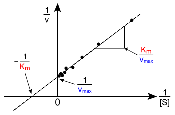
The Lineweaver–Burk plot was widely used to determine important terms in enzyme kinetics, such as Km and Vmax, before the wide availability of powerful computers and non-linear regression software. The y-intercept of such a graph is equivalent to the inverse of Vmax; the x-intercept of the graph represents −1/Km. It also gives a quick, visual impression of the different forms of enzyme inhibition.
The double reciprocal plot distorts the error structure of the data, and it is therefore unreliable for the determination of enzyme kinetic parameters. Although it is still used for representation of kinetic data,[2] non-linear regression or alternative linear forms of the Michaelis–Menten equation such as the Hanes-Woolf plot or Eadie–Hofstee plot are generally used for the calculation of parameters.[3]
When used for determining the type of enzyme inhibition, the Lineweaver–Burk plot can distinguish competitive, non-competitive and uncompetitive inhibitors. Competitive inhibitors have the same y-intercept as uninhibited enzyme (since Vmax is unaffected by competitive inhibitors the inverse of Vmax also doesn't change) but there are different slopes and x-intercepts between the two data sets. Non-competitive inhibition produces plots with the same x-intercept as uninhibited enzyme (Km is unaffected) but different slopes and y-intercepts. Uncompetitive inhibition causes different intercepts on both the y- and x-axes .
Problems with the method
The Lineweaver–Burk plot is classically used in older texts, but is prone to error, as the y-axis takes the reciprocal of the rate of reaction – in turn increasing any small errors in measurement. Also, most points on the plot are found far to the right of the y-axis. Large values of [S] (and hence small values for 1/[S] on the plot) are often not possible due to limited solubility, calling for a large extrapolation back to obtain x- and y-intercepts.[4]
References
- Lineweaver, H; Burk, D. (1934). "The determination of enzyme dissociation constants". Journal of the American Chemical Society. 56 (3): 658–666. doi:10.1021/ja01318a036.
- Hayakawa, K.; Guo, L.; Terentyeva, E.A.; Li, X.K.; Kimura, H.; Hirano, M.; Yoshikawa, K.; Nagamine, T.; et al. (2006). "Determination of specific activities and kinetic constants of biotinidase and lipoamidase in LEW rat and Lactobacillus casei (Shirota)". Journal of Chromatography B. 844 (2): 240–50. doi:10.1016/j.jchromb.2006.07.006. PMID 16876490.
- Greco, W.R.; Hakala, M.T. (1979). "Evaluation of methods for estimating the dissociation constant of tight binding enzyme inhibitors" (PDF). Journal of Biological Chemistry. 254 (23): 12104–12109. PMID 500698.
- Dowd, John E.; Riggs, Douglas S. (1965). "A comparison of estimates of Michaelis–Menten kinetic constants from various linear transformations" (pdf). Journal of Biological Chemistry. 240 (2): 863–869.
External links
- NIH guide, enzyme assay development and analysis