Line integral convolution

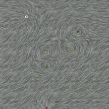
Intuitively, the flow of a vector field in some domain is visualized by adding a static random pattern of dark and light paint sources. As the flow passes by the sources, each parcel of fluid picks up some of the source color, averaging it with the color it has already acquired in a manner similar to throwing paint in a river. The result is a random striped texture where points along the same streamline tend to have similar color.

Algorithmically, the technique starts by generating in the domain of the vector field a random gray level image at the desired output resolution. Then, for every pixel in this image, the forward and backward streamline of a fixed arc length is calculated. The value assigned to the current pixel is computed by a convolution of a suitable convolution kernel with the gray levels of all the pixels lying on a segment of this streamline. This creates a gray level LIC image.

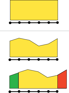
Although the input vector field and the result image are discretized, it pays to look at it from a continuous viewpoint.[2] Let ${\displaystyle \mathbf {v} }$ be the vector field given in some domain ${\displaystyle \Omega }$. Although the input vector field is typically discretized, we regard the field ${\displaystyle \mathbf {v} }$ as defined in every point of ${\displaystyle \Omega }$, i.e. we assume an interpolation. Streamlines, or more generally field lines, are tangent to the vector field in each point. They end either at the boundary of ${\displaystyle \Omega }$ or at critical points where ${\displaystyle \mathbf {v} =\mathbf {0} }$. For the sake of simplicity, in the following critical points and boundaries are ignored. A field line ${\displaystyle {\boldsymbol {\sigma }}}$, parametrized by arc length ${\displaystyle s}$, is defined as ${\displaystyle {\frac {d{\boldsymbol {\sigma }}(s)}{ds}}={\frac {\mathbf {v} ({\boldsymbol {\sigma }}(s))}{|\mathbf {v} ({\boldsymbol {\sigma }}(s))|}}}$. Let ${\displaystyle {\boldsymbol {\sigma }}_{\mathbf {r} }(s)}$ be the field line that passes through the point ${\displaystyle \mathbf {r} }$ for ${\displaystyle s=0}$. Then the image gray value at ${\displaystyle \mathbf {r} }$ is set to

${\displaystyle D(\mathbf {r} )=\int _{-L/2}^{L/2}k(s)N({\boldsymbol {\sigma }}_{\mathbf {r} }(s))ds}$

where ${\displaystyle k(s)}$ is the convolution kernel, ${\displaystyle N(\mathbf {r} )}$ is the noise image, and ${\displaystyle L}$ is the length of field line segment that is followed.

${\displaystyle D(\mathbf {r} )}$ has to be computed for each pixel in the LIC image. If carried out naively, this is quite expensive. First, the field lines have to be computed using a numerical method for solving ordinary differential equations, like a Runge–Kutta method, and then for each pixel the convolution along a field line segment has to be calculated. The computation can be significantly accelerated by re-using parts of already computed field lines, specializing to a box function as convolution kernel ${\displaystyle k(s)}$ and avoiding redundant computations during convolution.[2] The resulting fast LIC method can be generalized to convolution kernels that are arbitrary polynomials.[3]

Note that ${\displaystyle \Omega }$ does not have to be a 2D domain: the method is applicable to higher dimensional domains using multidimensional noise fields. However, the visualization of the higher-dimensional LIC texture is problematic; one way is to use interactive exploration with 2D slices that are manually positioned and rotated. The domain ${\displaystyle \Omega }$ does not have to be flat either; the LIC texture can be computed also for arbitrarily shaped 2D surfaces in 3D space.[4]

The output image will normally be colored in some way. Typically some scalar field in ${\displaystyle \Omega }$ is used, like the vector length, to determine the hue, while the gray-scale LIC image determines the brightness of the color.

Different choices of convolution kernels and random noise produce different textures: for example pink noise produces a cloudy pattern where areas of higher flow stand out as smearing, suitable for weather visualization. Further refinements in the convolution can improve the quality of the image.[5]

References

- Cabral, Brian; Leedom, Leith Casey (August 2–6, 1993). "Imaging Vector Fields Using Line Integral Convolution". Proceedings of the 20th annual conference on Computer graphics and interactive techniques. SIGGRAPH '93. Anaheim, California. pp. 263–270. CiteSeerX 10.1.1.115.1636. doi:10.1145/166117.166151. ISBN 0-89791-601-8.
- Stalling, Detlev; Hege, Hans-Christian (August 6–11, 1995). "Fast and Resolution Independent Line Integral Convolution". Proceedings of the 22nd Annual Conference on Computer Graphics and Interactive Techniques. SIGGRAPH '95. Los Angeles, California. pp. 249–256. CiteSeerX 10.1.1.45.5526. doi:10.1145/218380.218448. ISBN 0-89791-701-4.
- Hege, Hans-Christian; Stalling, Detlev (1998), "Fast LIC with piecewise polynomial filter kernels", in Hege, Hans-Christian; Polthier, Konrad (eds.), Mathematical Visualization, Berlin, Heidelberg: Springer-Verlag, pp. 295–314, CiteSeerX 10.1.1.31.504, doi:10.1007/978-3-662-03567-2_22, ISBN 978-3-642-08373-0
- Battke, Henrik; Stalling, Detlev; Hege, Hans-Christian (1997). "Fast Line Integral Convolution for Arbitrary Surfaces in 3D". In Hege, Hans-Christian; Polthier, Konrad (eds.). Visualization and Mathematics: Experiments, Simulations, and Environments. Berlin, New York: Springer. pp. 181–195. CiteSeerX 10.1.1.71.7228. doi:10.1007/978-3-642-59195-2_12. ISBN 3-540-61269-6.
- Weiskopf, Daniel (2009). "Iterative Twofold Line Integral Convolution for Texture-Based Vector Field Visualization". In Möller, Torsten; Hamann, Bernd; Russell, Robert D. (eds.). Mathematical Foundations of Scientific Visualization, Computer Graphics, and Massive Data Exploration. Mathematics and Visualization. Berlin, New York: Springer. pp. 191–211. CiteSeerX 10.1.1.66.3013. doi:10.1007/b106657_10. ISBN 978-3-540-25076-0.
- Shen, Han-Wei; Kam, David L. (1998). "A New Line Integral Convolution Algorithm for Visualizing Time-Varying Flow Fields" (PDF). IEEE Trans Vis Comput Graph. Los Alamitos: IEEE. 4 (2): 98–108. doi:10.1109/2945.694952. ISSN 1077-2626.
- Zöckler, Malte; Stalling, Detlev; Hege, Hans-Christian (1997). "Parallel Line Integral Convolution" (PDF). Parallel Computing. Amsterdam: North Holland. 23 (7): 975–989. doi:10.1016/S0167-8191(97)00039-2. ISSN 0167-8191.
- Ding, Zi'ang; Liu, Zhanping; Yu, Yang; Chen, Wei (2015). "Parallel unsteady flow line integral convolution for high-performance dense visualization". 2015 IEEE Pacific Visualization Symposium, PacificVis 2015. Hangzhou, China. pp. 25–30.
- Laidlaw, David H.; Kirby, Robert M.; Davidson, J. Scott; Miller, Timothy S.; da Silva, Marco; Warren, William H.; Tarr, Michael J. (October 21–26, 2001). "Quantitative Comparative Evaluation of 2D Vector Field Visualization Methods". IEEE Visualization 2001, VIS '01. Proceedings. San Diego, CA, USA. pp. 143–150.