Hann function

Top: 16 sample DFT-even Hann window. Bottom: Its discrete-time Fourier transform (DTFT) and the 3 non-zero values of its discrete Fourier transform (DFT).

The Hann window is a linear combination of modulated rectangular windows:

${\displaystyle \mathrm {rect} (x/L)\quad {\stackrel {\text{Fourier transform}}{\longleftrightarrow }}\quad L\cdot \mathrm {sinc} (Lf)={\frac {\sin(\pi Lf)}{\pi f}}.}$

Using Euler's formula to expand the cosine term, we can write:

${\displaystyle w_{0}(x)={\tfrac {1}{2}}\mathrm {rect} (x/L)+{\tfrac {1}{4}}e^{i2\pi x/L}\mathrm {rect} (x/L)+{\tfrac {1}{4}}e^{-i2\pi x/L}\mathrm {rect} (x/L),}$

whose Fourier transform is just:

${\displaystyle W_{0}(f)={\tfrac {1}{2}}{\frac {\sin(\pi Lf)}{\pi f}}+{\tfrac {1}{4}}{\frac {\sin(\pi L(f-1/L))}{\pi (f-1/L)}}+{\tfrac {1}{4}}{\frac {\sin(\pi L(f+1/L))}{\pi (f+1/L)}}.}$

The Discrete-time Fourier transform (DTFT) of the N+1 length, time-shifted sequence is defined by a Fourier series, which also has a 3-term equivalent that is derived similarly to the Fourier transform derivation:

${\displaystyle {\begin{aligned}{\mathcal {F}}\{w[n]\}&\triangleq \sum _{n=0}^{N}w[n]\cdot e^{-i2\pi fn}\\&=e^{-i\pi fN}\left[{\tfrac {1}{2}}{\frac {\sin(\pi (N+1)f)}{\sin(\pi f)}}+{\tfrac {1}{4}}{\frac {\sin(\pi (N+1)(f-{\tfrac {1}{N}}))}{\sin(\pi (f-{\tfrac {1}{N}}))}}+{\tfrac {1}{4}}{\frac {\sin(\pi (N+1)(f+{\tfrac {1}{N}}))}{\sin(\pi (f+{\tfrac {1}{N}}))}}\right].\end{aligned}}}$

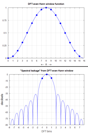
For even values of N, the truncated sequence ${\displaystyle \{w[n],\ 0\leq n\leq N-1\}}$ is a DFT-even (aka periodic) Hann window. Since the truncated sample has value zero, it is clear from the Fourier series definition that the DTFTs are equivalent. However, the approach followed above results in a significantly different-looking, but equivalent, 3-term expression:

${\displaystyle {\mathcal {F}}\{w[n]\}=e^{-i\pi f(N-1)}\left[{\tfrac {1}{2}}{\frac {\sin(\pi Nf)}{\sin(\pi f)}}+{\tfrac {1}{4}}e^{-i\pi /N}{\frac {\sin(\pi N(f-{\tfrac {1}{N}}))}{\sin(\pi (f-{\tfrac {1}{N}}))}}+{\tfrac {1}{4}}e^{i\pi /N}{\frac {\sin(\pi N(f+{\tfrac {1}{N}}))}{\sin(\pi (f+{\tfrac {1}{N}}))}}\right].}$

An N-length DFT of the window function samples the DTFT at frequencies ${\displaystyle f=k/N,}$ for integer values of ${\displaystyle k.}$ From the expression immediately above, it is easy to see that only 3 of the N DFT coefficients are non-zero. And from the other expression, it is apparent that all are real-valued. These properties are appealing for real-time applications that require both windowed and non-windowed (rectangularly windowed) transforms, because the windowed transforms can be efficiently derived from the non-windowed transforms by convolution.[5]

The function is named in honour of von Hann, who used the three-term weighted average smoothing technique on meteorological data.[6][3] However, the erroneous[2] "Hanning" function is also heard of on occasion, derived from the paper in which it was named, where the term "hanning a signal" was used to mean applying the Hann window to it.[7][8] The confusion arose from the similar Hamming function, named after Richard Hamming.

• Window function
• Apodization
• Raised cosine distribution
• Raised-cosine filter

• Hann function at MathWorld

References

- Essenwanger, O. M. (Oskar M.) (1986). Elements of statistical analysis. Elsevier. ISBN 0444424261. OCLC 152410575.
- Harris, Fredric J. (Jan 1978). "On the use of Windows for Harmonic Analysis with the Discrete Fourier Transform" (PDF). Proceedings of the IEEE. 66 (1): 51–83. CiteSeerX 10.1.1.649.9880. doi:10.1109/PROC.1978.10837.
The correct name of this window is “Hann.” The term “Hanning” is used in this report to reflect conventional usage. The derived term “Hann’d” is also widely used.
- Kahlig, Peter (1993), "Some aspects of Julius von Hann's contribution to modern climatology", in McBean, G.A.; Hantel, M. (eds.), Interactions Between Global Climate Subsystems: The Legacy of Hann, Geophysical Monograph Series, 75, American Geophysical Union, pp. 1–7, doi:10.1029/gm075p0001, ISBN 9780875904665, retrieved 2019-07-01,
Hann appears to be the inventor of a certain data smoothing procedure, now called "hanning" ... or "Hann smoothing" ... Essentially, it is a three-term moving average (running mean) with unequal weights (1/4, 1/2, 1/4).
- Smith, Julius O. (Julius Orion) (2011). Spectral audio signal processing. Stanford University. Center for Computer Research in Music and Acoustics., Stanford University. Department of Music. [Stanford, Calif.?]: W3K. ISBN 9780974560731. OCLC 776892709.
- US patent 6898235, Carlin, Joe; Terry Collins & Peter Hays et al., "Wideband communication intercept and direction finding device using hyperchannelization", issued 2005
- Hann, Julius von (1903). Handbook of Climatology. Macmillan. p. 199.
The figures under b are determined by taking into account the parallels 5° away on either side. Thus, for example, for latitude 60° we have ½[60+(65+55)÷2].
- Blackman, R. B.; Tukey, J. W. (1958). "The measurement of power spectra from the point of view of communications engineering — Part I". The Bell System Technical Journal. 37 (1): 273. doi:10.1002/j.1538-7305.1958.tb03874.x. ISSN 0005-8580.
- Blackman, R. B. (Ralph Beebe); Tukey, John W. (John Wilder) (1959). The measurement of power spectra from the point of view of communications engineering. New York : Dover Publications. pp. 98. LCCN 59-10185.