Lasso (statistics)

Some basic properties of the lasso estimator can now be considered.

Assuming first that the covariates are orthonormal so that ${\displaystyle (x_{i}\mid x_{j})=\delta _{ij}}$, where ${\displaystyle (\cdot \mid \cdot )}$ is the inner product and ${\displaystyle \delta _{ij}}$ is the Kronecker delta, or, equivalently, ${\displaystyle X^{T}X=I}$, then using subgradient methods it can be shown that

${\displaystyle {\begin{aligned}{\hat {\beta }}_{j}={}&S_{N\lambda }({\hat {\beta }}_{j}^{\text{OLS}})={\hat {\beta }}_{j}^{\text{OLS}}\max \left(0,1-{\frac {N\lambda }{|{\hat {\beta }}_{j}^{\text{OLS}}|}}\right)\\&{\text{ where }}{\hat {\beta }}^{\text{OLS}}=(X^{T}X)^{-1}X^{T}y\end{aligned}}}$ [2]

${\displaystyle S_{\alpha }}$ is referred to as the soft thresholding operator, since it translates values towards zero (making them exactly zero if they are small enough) instead of setting smaller values to zero and leaving larger ones untouched as the hard thresholding operator, often denoted ${\displaystyle H_{\alpha }}$, would.

This can be compared to ridge regression, where the objective is to minimize

${\displaystyle \min _{\beta \in \mathbb {R} ^{p}}\left\{{\frac {1}{N}}\|y-X\beta \|_{2}^{2}+\lambda \|\beta \|_{2}^{2}\right\}}$

yielding

${\displaystyle {\hat {\beta }}_{j}=(1+N\lambda )^{-1}{\hat {\beta }}_{j}^{\text{OLS}}.}$

So ridge regression shrinks all coefficients by a uniform factor of ${\displaystyle (1+N\lambda )^{-1}}$ and does not set any coefficients to zero.

It can also be compared to regression with best subset selection, in which the goal is to minimize

${\displaystyle \min _{\beta \in \mathbb {R} ^{p}}\left\{{\frac {1}{N}}\left\|y-X\beta \right\|_{2}^{2}+\lambda \|\beta \|_{0}\right\}}$

where ${\displaystyle \|\cdot \|_{0}}$ is the "${\displaystyle \ell ^{0}}$ norm", which is defined as ${\displaystyle \|z\|=m}$ if exactly m components of z are nonzero. In this case, it can be shown that

${\displaystyle {\hat {\beta }}_{j}=H_{\sqrt {N\lambda }}\left({\hat {\beta }}_{j}^{\text{OLS}}\right)={\hat {\beta }}_{j}^{\text{OLS}}\mathrm {I} \left(\left|{\hat {\beta }}_{j}^{\text{OLS}}\right|\geq {\sqrt {N\lambda }}\right)}$

where ${\displaystyle H_{\alpha }}$ is the so-called hard thresholding function and ${\displaystyle \mathrm {I} }$ is an indicator function (it is 1 if its argument is true and 0 otherwise).

Therefore, the lasso estimates share features of the estimates from both ridge and best subset selection regression since they both shrink the magnitude of all the coefficients, like ridge regression, but also set some of them to zero, as in the best subset selection case. Additionally, while ridge regression scales all of the coefficients by a constant factor, lasso instead translates the coefficients towards zero by a constant value and sets them to zero if they reach it.

Returning to the general case, in which the different covariates may not be independent, a special case may be considered in which two of the covariates, say j and k, are identical for each case, so that ${\displaystyle x_{(j)}=x_{(k)}}$, where ${\displaystyle x_{(j),i}=x_{(k),i}}$. Then the values of ${\displaystyle \beta _{j}}$ and ${\displaystyle \beta _{k}}$ that minimize the lasso objective function are not uniquely determined. In fact, if there is some solution ${\displaystyle {\hat {\beta }}}$ in which ${\displaystyle {\hat {\beta }}_{j}{\hat {\beta }}_{k}\geq 0}$, then if ${\displaystyle s\in [0,1]}$ replacing ${\displaystyle {\hat {\beta }}_{j}}$ by ${\displaystyle s({\hat {\beta }}_{j}+{\hat {\beta }}_{k})}$ and ${\displaystyle {\hat {\beta }}_{k}}$ by ${\displaystyle (1-s)({\hat {\beta }}_{j}+{\hat {\beta }}_{k})}$, while keeping all the other ${\displaystyle {\hat {\beta }}_{i}}$ fixed, gives a new solution, so the lasso objective function then has a continuum of valid minimizers.[6] Several variants of the lasso, including the Elastic Net, have been designed to address this shortcoming, which are discussed below.

Forms of the constraint regions for lasso and ridge regression.

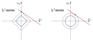
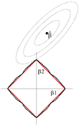
As discussed above, lasso can set coefficients to zero, while ridge regression, which appears superficially similar, cannot. This is due to the difference in the shape of the constraint boundaries in the two cases. Both lasso and ridge regression can be interpreted as minimizing the same objective function

${\displaystyle \min _{\beta _{0},\beta }\left\{{\frac {1}{N}}\left\|y-\beta _{0}-X\beta \right\|_{2}^{2}\right\}}$

but with respect to different constraints: ${\displaystyle \|\beta \|_{1}\leq t}$ for lasso and ${\displaystyle \|\beta \|_{2}^{2}\leq t}$ for ridge. From the figure, one can see that the constraint region defined by the ${\displaystyle \ell ^{1}}$ norm is a square rotated so that its corners lie on the axes (in general a cross-polytope), while the region defined by the ${\displaystyle \ell ^{2}}$ norm is a circle (in general an n-sphere), which is rotationally invariant and, therefore, has no corners. As seen in the figure, a convex object that lies tangent to the boundary, such as the line shown, is likely to encounter a corner (or a higher-dimensional equivalent) of a hypercube, for which some components of ${\displaystyle \beta }$ are identically zero, while in the case of an n-sphere, the points on the boundary for which some of the components of ${\displaystyle \beta }$ are zero are not distinguished from the others and the convex object is no more likely to contact a point at which some components of ${\displaystyle \beta }$ are zero than one for which none of them are.

The lasso can be rescaled so that it becomes easy to anticipate and influence what degree of shrinkage is associated with a given value of ${\displaystyle \lambda }$ (Hoornweg, 2018). It is assumed that ${\displaystyle X}$ is standardized with z-scores and that ${\displaystyle y}$ is centered so that it has a mean of zero. Let ${\displaystyle \beta _{0}}$ represent the hypothesized regression coefficients and let ${\displaystyle b_{OLS}}$ refer to the data-optimized ordinary least squares solutions. We can then define the Lagrangian as a tradeoff between the in-sample accuracy of the data-optimized solutions and the simplicity of sticking to the hypothesized values. This results in

${\displaystyle \min _{\beta \in \mathbb {R} ^{p}}\left\{{\frac {(y-X\beta )'(y-X\beta )}{(y-X\beta _{0})'(y-X\beta _{0})}}+2\lambda \sum _{i=1}^{p}{\frac {|\beta _{i}-\beta _{0,i}|}{q_{i}}}\right\}}$

where ${\displaystyle q_{i}}$ is specified below. The first fraction represents relative accuracy, the second fraction relative simplicity, and ${\displaystyle \lambda }$ balances between the two.

Stylized solution paths for the ${\displaystyle \ell _{1}}$ norm and ${\displaystyle \ell _{2}}$ norm when ${\displaystyle b_{OLS}=2}$ and ${\displaystyle \beta _{0}=0}$

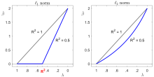
If there is a single regressor, then relative simplicity can be defined by specifying ${\displaystyle q_{i}}$ as ${\displaystyle |b_{OLS}-\beta _{0}|}$, which is the maximum amount of deviation from ${\displaystyle \beta _{0}}$ when ${\displaystyle \lambda =0}$. Assuming that ${\displaystyle \beta _{0}=0}$, the solution path can then be defined in terms of the famous accuracy measure called ${\displaystyle R^{2}}$:

${\displaystyle b_{\ell _{1}}={\begin{cases}(1-\lambda /R^{2})b_{OLS}&{\mbox{if }}\lambda \leq R^{2},\\0&{\mbox{if }}\lambda >R^{2}.\end{cases}}}$

If ${\displaystyle \lambda =0}$, the OLS solution is used. The hypothesized value of ${\displaystyle \beta _{0}=0}$ is selected if ${\displaystyle \lambda }$ is bigger than ${\displaystyle R^{2}}$. Furthermore, if ${\displaystyle R^{2}=1}$, then ${\displaystyle \lambda }$ represents the proportional influence of ${\displaystyle \beta _{0}=0}$. In other words, ${\displaystyle \lambda \times 100\%}$ measures in percentage terms what the minimal amount of influence is of the hypothesized value relative to the data-optimized OLS solution.

If an ${\displaystyle \ell _{2}}$-norm is used to penalize deviations from zero when there is a single regressor, the solution path is given by ${\displaystyle b_{\ell _{2}}={\bigg (}1+{\frac {\lambda }{R^{2}(1-\lambda )}}{\bigg )}^{-1}b_{OLS}}$. Like ${\displaystyle b_{\ell _{1}}}$, ${\displaystyle b_{\ell _{2}}}$ moves in the direction of the point ${\displaystyle (\lambda =R^{2},b=0)}$ when ${\displaystyle \lambda }$ is close to zero; but unlike ${\displaystyle b_{\ell _{1}}}$, the influence of ${\displaystyle R^{2}}$ diminishes in ${\displaystyle b_{\ell _{2}}}$ if ${\displaystyle \lambda }$ increases (see figure).

When there are multiple regressors, the moment that a parameter is activated (i.e. allowed to deviate from ${\displaystyle \beta _{0}}$) is also determined by a regressor's contribution to ${\displaystyle R^{2}}$ accuracy. First, we define

${\displaystyle R^{2}=1-{\frac {(y-Xb)'(y-Xb)}{(y-X\beta _{0})'(y-X\beta _{0})}}.}$

An ${\displaystyle R^{2}}$ of 75% means that the in-sample accuracy improves by 75% if the unrestricted OLS solutions are used instead of the hypothesized ${\displaystyle \beta _{0}}$ values. The individual contribution of deviating from each hypothesis can be computed with the ${\displaystyle p}$ times ${\displaystyle p}$ matrix

${\displaystyle R^{\otimes }=(X'{\tilde {y}}_{0})(X'{\tilde {y}}_{0})'(X'X)^{-1}({\tilde {y}}_{0}'{\tilde {y}}_{0})^{-1},}$

where ${\displaystyle {\tilde {y}}_{0}=y-X\beta _{0}}$. If ${\displaystyle b=b_{OLS}}$ when ${\displaystyle R^{2}}$ is computed, then the diagonal elements of ${\displaystyle R^{\otimes }}$ sum to ${\displaystyle R^{2}}$. The diagonal ${\displaystyle R^{\otimes }}$ values may be smaller than 0 and, in more exceptional cases, larger than 1. If regressors are uncorrelated, then the ${\displaystyle i^{th}}$ diagonal element of ${\displaystyle R^{\otimes }}$ simply corresponds to the ${\displaystyle r^{2}}$ value between ${\displaystyle x_{i}}$ and ${\displaystyle y}$.

Now, we can obtain a rescaled version of the adaptive lasso of Zou (2006) by setting ${\displaystyle q_{{\mbox{adaptive lasso}},i}=|b_{OLS,i}-\beta _{0,i}|}$. If regressors are uncorrelated, the moment that the ${\displaystyle i^{th}}$ parameter is activated is given by the ${\displaystyle i^{th}}$ diagonal element of ${\displaystyle R^{\otimes }}$. If we also assume for convenience that ${\displaystyle \beta _{0}}$ is a vector of zeros, we get

${\displaystyle b_{i}={\begin{cases}(1-\lambda /R_{ii}^{\otimes })b_{OLS,i}&{\mbox{if }}\lambda \leq R_{ii}^{\otimes },\\0&{\mbox{if }}\lambda >R_{ii}^{\otimes }.\end{cases}}}$

That is, if regressors are uncorrelated, ${\displaystyle \lambda }$ again specifies what the minimal influence of ${\displaystyle \beta _{0}}$ is. Even when regressors are correlated, moreover, the first time that a regression parameter is activated occurs when ${\displaystyle \lambda }$ is equal to the highest diagonal element of ${\displaystyle R^{\otimes }}$.

These results can be compared to a rescaled version of the lasso if we define ${\displaystyle q_{{\mbox{lasso}},i}={\frac {1}{p}}\sum _{l}|b_{OLS,l}-\beta _{0,l}|}$, which is the average absolute deviation of ${\displaystyle b_{OLS}}$ from ${\displaystyle \beta _{0}}$. If we assume that regressors are uncorrelated, then the moment of activation of the ${\displaystyle i^{th}}$ regressor is given by

${\displaystyle {\tilde {\lambda }}_{{\text{lasso}},i}={\frac {1}{p}}{\sqrt {R_{i}^{\otimes }}}\sum _{l=1}^{p}{\sqrt {R_{l}^{\otimes }}}.}$

For ${\displaystyle p=1}$, the moment of activation is again given by ${\displaystyle {\tilde {\lambda }}_{{\text{lasso}},i}=R^{2}}$. Moreover, if ${\displaystyle \beta _{0}}$ is a vector of zeros and there is a subset of ${\displaystyle p_{B}}$ relevant parameters that are equally responsible for a perfect fit of ${\displaystyle R^{2}=1}$, then this subset will be activated at a ${\displaystyle \lambda }$ value of ${\displaystyle {\frac {1}{p}}}$. After all, the moment of activation of a relevant regressor then equals ${\displaystyle {\frac {1}{p}}{\frac {1}{\sqrt {p_{B}}}}p_{B}{\frac {1}{\sqrt {p_{B}}}}={\frac {1}{p}}}$. In other words, the inclusion of irrelevant regressors delays the moment that relevant regressors are activated by this rescaled lasso. The adaptive lasso and the lasso are special cases of a '1ASTc' estimator. The latter only groups parameters together if the absolute correlation among regressors is larger than a user-specified value. For further details, see Hoornweg (2018).[7]

Laplace distributions are sharply peaked at their mean with more probability density concentrated there compared to a normal distribution.

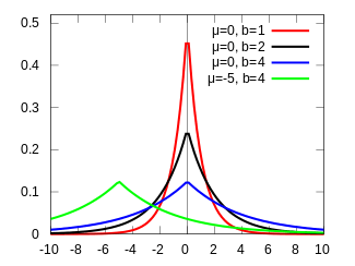
Just as ridge regression can be interpreted as linear regression for which the coefficients have been assigned normal prior distributions, lasso can be interpreted as linear regression for which the coefficients have Laplace prior distributions. The Laplace distribution is sharply peaked at zero (its first derivative is discontinuous) and it concentrates its probability mass closer to zero than does the normal distribution. This provides an alternative explanation of why lasso tends to set some coefficients to zero, while ridge regression does not.[2]

Lasso can also be viewed as a convex relaxation of the best subset selection regression problem, which is to find the subset of ${\displaystyle \leq k}$ covariates that results in the smallest value of the objective function for some fixed ${\displaystyle k\leq n}$, where n is the total number of covariates. The "${\displaystyle \ell ^{0}}$ norm", ${\displaystyle \|\cdot \|_{0}}$, which gives the number of nonzero entries of a vector, is the limiting case of "${\displaystyle \ell ^{p}}$ norms", of the form ${\displaystyle \textstyle \|x\|_{p}=\left(\sum _{i=1}^{n}|x_{j}|^{p}\right)^{1/p}}$ (where the quotation marks signify that these are not really norms for ${\displaystyle p<1}$ since ${\displaystyle \|\cdot \|_{p}}$ is not convex for ${\displaystyle p<1}$, so the triangle inequality does not hold). Therefore, since p = 1 is the smallest value for which the "${\displaystyle \ell ^{p}}$ norm" is convex (and therefore actually a norm), lasso is, in some sense, the best convex approximation to the best subset selection problem, since the region defined by ${\displaystyle \|x\|_{1}\leq t}$ is the convex hull of the region defined by ${\displaystyle \|x\|_{p}\leq t}$ for ${\displaystyle p<1}$.

In 2005, Zou and Hastie introduced the elastic net to address several shortcomings of lasso.[6] When p > n (the number of covariates is greater than the sample size) lasso can select only n covariates (even when more are associated with the outcome) and it tends to select only one covariate from any set of highly correlated covariates. Additionally, even when n > p, if the covariates are strongly correlated, ridge regression tends to perform better.

The elastic net extends lasso by adding an additional ${\displaystyle \ell ^{2}}$ penalty term giving

${\displaystyle \min _{\beta \in \mathbb {R} ^{p}}\left\{\left\|y-X\beta \right\|_{2}^{2}+\lambda _{1}\|\beta \|_{1}+\lambda _{2}\|\beta \|_{2}^{2}\right\},}$

which is equivalent to solving

${\displaystyle {\begin{aligned}\min _{\beta _{0},\beta }\left\{\left\|y-\beta _{0}-X\beta \right\|_{2}^{2}\right\}&{\text{ subject to }}(1-\alpha )\|\beta \|_{1}+\alpha \|\beta \|_{2}^{2}\leq t,\\&{\text{ where }}\alpha ={\frac {\lambda _{2}}{\lambda _{1}+\lambda _{2}}}.\end{aligned}}}$

Somewhat surprisingly, this problem can be written in a simple lasso form

${\displaystyle \min _{\beta ^{*}\in \mathbb {R} ^{p}}\left\{\left\|y^{*}-X^{*}\beta ^{*}\right\|_{2}^{2}+\lambda ^{*}\|\beta ^{*}\|_{1}\right\}}$

letting

${\displaystyle X_{(n+p)\times p}^{*}=(1+\lambda _{2})^{-1/2}{\binom {X}{\lambda _{2}^{1/2}I_{p\times p}}}}$,   ${\displaystyle y_{(n+p)}^{*}={\binom {y}{0^{p}}},\qquad \lambda ^{*}={\frac {\lambda _{1}}{\sqrt {1+\lambda _{2}}}}}$,   ${\displaystyle \beta ^{*}={\sqrt {1+\lambda _{2}}}\beta .}$

Then ${\displaystyle {\hat {\beta }}={\frac {{\hat {\beta }}^{*}}{\sqrt {1+\lambda _{2}}}}}$, which, when the covariates are orthogonal to each other, gives

${\displaystyle {\hat {\beta }}_{j}={\frac {{\hat {\beta }}_{j}^{\text{*,OLS}}}{\sqrt {1+\lambda _{2}}}}\max \left(0,1-{\frac {\lambda ^{*}}{\left|{\hat {\beta }}_{j}^{\text{*,OLS}}\right|}}\right)={\frac {{\hat {\beta }}_{j}^{\text{OLS}}}{1+\lambda _{2}}}\max \left(0,1-{\frac {\lambda _{1}}{\left|{\hat {\beta }}_{j}^{\text{OLS}}\right|}}\right)=(1+\lambda _{2})^{-1}{\hat {\beta }}_{j}^{\text{lasso}}.}$

So the result of the elastic net penalty is a combination of the effects of the lasso and Ridge penalties.

Returning to the general case, the fact that the penalty function is now strictly convex means that if ${\displaystyle x_{(j)}=x_{(k)}}$, ${\displaystyle {\hat {\beta }}_{j}={\hat {\beta }}_{k}}$, which is a change from lasso.[6] In general, if ${\displaystyle {\hat {\beta }}_{j}{\hat {\beta _{k}}}>0}$

${\displaystyle {\frac {|{\hat {\beta }}_{j}-{\hat {\beta _{k}}}|}{\|y\|}}\leq \lambda _{2}^{-1}{\sqrt {2(1-\rho _{jk})}},{\text{ where }}\rho =X^{t}X,}$

is the sample correlation matrix because the ${\displaystyle x}$ 's are normalized.

Therefore, highly correlated covariates will tend to have similar regression coefficients, with the degree of similarity depending on both ${\displaystyle \|y\|_{1}}$ and ${\displaystyle \lambda _{2}}$, which is very different from lasso. This phenomenon, in which strongly correlated covariates have similar regression coefficients, is referred to as the grouping effect and is generally considered desirable since, in many applications, such as identifying genes associated with a disease, one would like to find all the associated covariates, rather than selecting only one from each set of strongly correlated covariates, as lasso often does.[6] In addition, selecting only a single covariate from each group will typically result in increased prediction error, since the model is less robust (which is why ridge regression often outperforms lasso).

In 2006, Yuan and Lin introduced the group lasso in order to allow predefined groups of covariates to be selected into or out of a model together, where all the members of a particular group are either included or not included.[8] While there are many settings in which this is useful, perhaps the most obvious is when levels of a categorical variable are coded as a collection of binary covariates. In this case, it often doesn't make sense to include only a few levels of the covariate; the group lasso can ensure that all the variables encoding the categorical covariate are either included or excluded from the model together. Another setting in which grouping is natural is in biological studies. Since genes and proteins often lie in known pathways, an investigator may be more interested in which pathways are related to an outcome than whether particular individual genes are. The objective function for the group lasso is a natural generalization of the standard lasso objective

${\displaystyle \min _{\beta \in \mathbb {R} ^{p}}\left\{\left\|y-\sum _{j=1}^{J}X_{j}\beta _{j}\right\|_{2}^{2}+\lambda \sum _{j=1}^{J}\|\beta _{j}\|_{K_{j}}\right\},\qquad \|z\|_{K_{j}}=(z^{t}K_{j}z)^{1/2}}$

where the design matrix ${\displaystyle X}$ and covariate vector ${\displaystyle \beta }$ have been replaced by a collection of design matrices ${\displaystyle X_{j}}$ and covariate vectors ${\displaystyle \beta _{j}}$, one for each of the J groups. Additionally, the penalty term is now a sum over ${\displaystyle \ell ^{2}}$ norms defined by the positive definite matrices ${\displaystyle K_{j}}$. If each covariate is in its own group and ${\displaystyle K_{j}=I}$, then this reduces to the standard lasso, while if there is only a single group and ${\displaystyle K_{1}=I}$, it reduces to ridge regression. Since the penalty reduces to an ${\displaystyle \ell ^{2}}$ norm on the subspaces defined by each group, it cannot select out only some of the covariates from a group, just as ridge regression cannot. However, because the penalty is the sum over the different subspace norms, as in the standard lasso, the constraint has some non-differential points, which correspond to some subspaces being identically zero. Therefore, it can set the coefficient vectors corresponding to some subspaces to zero, while only shrinking others. However, it is possible to extend the group lasso to the so-called sparse group lasso, which can select individual covariates within a group, by adding an additional ${\displaystyle \ell ^{1}}$ penalty to each group subspace.[9] Another extension, group lasso with Overlap allows covariates to be shared between different groups, e.g. if a gene were to occur in two pathways.[10]

In some cases, the object being studied may have important spatial or temporal structure that must be accounted for during analysis, such as time series or image based data. In 2005, Tibshirani and colleagues introduced the fused lasso to extend the use of lasso to exactly this type of data.[11] The fused lasso objective function is

${\displaystyle {\begin{aligned}&\min _{\beta }\left\{{\frac {1}{N}}\sum _{i=1}^{N}\left(y_{i}-x_{i}^{t}\beta \right)^{2}\right\}\\[4pt]&{\text{ subject to }}\sum _{j=1}^{p}|\beta _{j}|\leq t_{1}{\text{ and }}\sum _{j=2}^{p}|\beta _{j}-\beta _{j-1}|\leq t_{2}.\end{aligned}}}$

The first constraint is just the typical lasso constraint, but the second directly penalizes large changes with respect to the temporal or spatial structure, which forces the coefficients to vary in a smooth fashion that reflects the underlying logic of the system being studied. Clustered lasso[12] is a generalization to fused lasso that identifies and groups relevant covariates based on their effects (coefficients). The basic idea is to penalize the differences between the coefficients so that nonzero ones make clusters together. This can be modeled using the following regularization:

${\displaystyle \sum _{i<j}^{p}|\beta _{i}-\beta _{j}|\leq t_{2}.}$

In contrast, one can first cluster variables into highly correlated groups, and then extract a single representative covariate from each cluster.[13]

Several algorithms exist that solve the fused lasso problem, and some generalizations of, in a direct form, i.e., there are algorithm that solve it exactly in a finite number of operations.[14]

An example of a PQSQ (piece-wise quadratic function of subquadratic growth) potential function ${\displaystyle u(x)}$; here the majorant function is ${\displaystyle f(x)=x}$; the potential is defined with trimming after ${\displaystyle r_{3}}$.

An example how efficient PQSQ regularized regression works just as ${\displaystyle \ell ^{1}}$-norm lasso.[15]

Lasso, elastic net, group and fused lasso construct the penalty functions from the ${\displaystyle \ell ^{1}}$ and ${\displaystyle \ell ^{2}}$ norms (with weights, if necessary). The bridge regression utilises general ${\displaystyle \ell ^{p}}$ norms (${\displaystyle p\geq 1}$) and quasinorms (${\displaystyle 0<p<1}$).[16] For example, for p=1/2 the analogue of lasso objective in the Lagrangian form is to solve

${\displaystyle \min _{\beta \in \mathbb {R} ^{p}}\left\{{\frac {1}{N}}\left\|y-X\beta \right\|_{2}^{2}+\lambda {\sqrt {\|\beta \|_{1/2}}}\right\},}$

where

${\displaystyle \|\beta \|_{1/2}=\left(\sum _{j=1}^{p}{\sqrt {|\beta _{j}|}}\right)^{2}}$

It is claimed that the fractional quasi-norms ${\displaystyle \ell ^{p}}$ (${\displaystyle 0<p<1}$) provide more meaningful results in data analysis both from the theoretical and empirical perspective.[17] But non-convexity of these quasi-norms causes difficulties in solution of the optimization problem. To solve this problem, an expectation-minimization procedure is developed[18] and implemented[15] for minimization of function

${\displaystyle \min _{\beta \in \mathbb {R} ^{p}}\left\{{\frac {1}{N}}\left\|y-X\beta \right\|_{2}^{2}+\lambda \sum _{j=1}^{p}\vartheta (\beta _{j}^{2})\right\},}$

where ${\displaystyle \vartheta (\gamma )}$ is an arbitrary concave monotonically increasing function (for example, ${\displaystyle \vartheta (\gamma )={\sqrt {\gamma }}}$ gives the lasso penalty and ${\displaystyle \vartheta (\gamma )=\gamma ^{1/4}}$ gives the ${\displaystyle \ell ^{1/2}}$ penalty).

The efficient algorithm for minimization is based on piece-wise quadratic approximation of subquadratic growth (PQSQ).[18]

The adaptive lasso was introduced by Zou (2006, JASA) for linear regression and by Zhang and Lu (2007, Biometrika) for proportional hazards regression.

The prior lasso was introduced by Jiang et al. (2016) for generalized linear models to incorporate prior information, such as the importance of certain covariates.[19] In prior lasso, such information is summarized into pseudo responses (called prior responses) ${\displaystyle {\hat {y}}^{\mathrm {p} }}$ and then an additional criterion function is added to the usual objective function of the generalized linear models with a lasso penalty. Without loss of generality, we use linear regression to illustrate prior lasso. In linear regression, the new objective function can be written as

${\displaystyle \min _{\beta \in \mathbb {R} ^{p}}\left\{{\frac {1}{N}}\left\|y-X\beta \right\|_{2}^{2}+{\frac {1}{N}}\eta \left\|{\hat {y}}^{\mathrm {p} }-X\beta \right\|_{2}^{2}+\lambda \|\beta \|_{1}\right\},}$

which is equivalent to

${\displaystyle \min _{\beta \in \mathbb {R} ^{p}}\left\{{\frac {1}{N}}\left\|{\tilde {y}}-X\beta \right\|_{2}^{2}+{\frac {\lambda }{1+\eta }}\|\beta \|_{1}\right\},}$

the usual lasso objective function with the responses ${\displaystyle y}$ being replaced by a weighted average of the observed responses and the prior responses ${\displaystyle {\tilde {y}}=(y+\eta {\hat {y}}^{\mathrm {p} })/(1+\eta )}$ (called the adjusted response values by the prior information).

In prior lasso, the parameter ${\displaystyle \eta }$ is called a balancing parameter, which balances the relative importance of the data and the prior information. In the extreme case of ${\displaystyle \eta =0}$, prior lasso is reduced to lasso. If ${\displaystyle \eta =\infty }$, prior lasso will solely rely on the prior information to fit the model. Furthermore, the balancing parameter ${\displaystyle \eta }$ has another appealing interpretation: it controls the variance of ${\displaystyle \beta }$ in its prior distribution from a Bayesian viewpoint.

Prior lasso is more efficient in parameter estimation and prediction (with a smaller estimation error and prediction error) when the prior information is of high quality, and is robust to the low quality prior information with a good choice of the balancing parameter ${\displaystyle \eta }$.

References

- Santosa, Fadil; Symes, William W. (1986). "Linear inversion of band-limited reflection seismograms". SIAM Journal on Scientific and Statistical Computing. SIAM. 7 (4): 1307–1330. doi:10.1137/0907087.
- Tibshirani, Robert (1996). "Regression Shrinkage and Selection via the lasso". Journal of the Royal Statistical Society. Series B (methodological). Wiley. 58 (1): 267–88. JSTOR 2346178.
- Tibshirani, Robert (1997). "The lasso Method for Variable Selection in the Cox Model". Statistics in Medicine. 16 (4): 385–395. CiteSeerX 10.1.1.411.8024. doi:10.1002/(SICI)1097-0258(19970228)16:4<385::AID-SIM380>3.0.CO;2-3. PMID 9044528.
- Breiman, Leo (1995). "Better Subset Regression Using the Nonnegative Garrote". Technometrics. 37 (4): 373–84. doi:10.1080/00401706.1995.10484371.
- Zou, Hui; Hastie, Trevor (2005). "Regularization and Variable Selection via the Elastic Net". Journal of the Royal Statistical Society. Series B (statistical Methodology). Wiley. 67 (2): 301–20. doi:10.1111/j.1467-9868.2005.00503.x. JSTOR 3647580.
- Hoornweg, Victor (2018). "Chapter 8". Science: Under Submission. Hoornweg Press. ISBN 978-90-829188-0-9.
- Yuan, Ming; Lin, Yi (2006). "Model Selection and Estimation in Regression with Grouped Variables". Journal of the Royal Statistical Society. Series B (statistical Methodology). Wiley. 68 (1): 49–67. doi:10.1111/j.1467-9868.2005.00532.x. JSTOR 3647556.
- Puig, Arnau Tibau, Ami Wiesel, and Alfred O. Hero. "A Multidimensional Shrinkage-Thresholding Operator". Proceedings of the 15th workshop on Statistical Signal Processing, SSP’09, IEEE, pp. 113–116.
- Jacob, Laurent, Guillaume Obozinski, and Jean-Philippe Vert. "Group Lasso with Overlap and Graph LASSO". Appearing in Proceedings of the 26th International Conference on Machine Learning, Montreal, Canada, 2009.
- Tibshirani, Robert, Michael Saunders, Saharon Rosset, Ji Zhu, and Keith Knight. 2005. “Sparsity and Smoothness via the Fused lasso”. Journal of the Royal Statistical Society. Series B (statistical Methodology) 67 (1). Wiley: 91–108. https://www.jstor.org/stable/3647602.
- She, Yiyuan (2010). "Sparse regression with exact clustering". Electronic Journal of Statistics. 4: 1055–1096. doi:10.1214/10-EJS578.
- Reid, Stephen (2015). "Sparse regression and marginal testing using cluster prototypes". Biostatistics. 17 (2): 364–76. arXiv:1503.00334. Bibcode:2015arXiv150300334R. doi:10.1093/biostatistics/kxv049. PMC 5006118. PMID 26614384.
- Bento, Jose (2018). "On the Complexity of the Weighted Fused Lasso". IEEE Letters in Signal Processing. 25 (10): 1595–1599. arXiv:1801.04987. Bibcode:2018ISPL...25.1595B. doi:10.1109/LSP.2018.2867800.
- Mirkes E.M. PQSQ-regularized-regression repository, GitHub.
- Fu, Wenjiang J. 1998. “The Bridge versus the Lasso”. Journal of Computational and Graphical Statistics 7 (3). Taylor & Francis: 397-416.
- Aggarwal C.C., Hinneburg A., Keim D.A. (2001) "On the Surprising Behavior of Distance Metrics in High Dimensional Space." In: Van den Bussche J., Vianu V. (eds) Database Theory — ICDT 2001. ICDT 2001. Lecture Notes in Computer Science, Vol. 1973. Springer, Berlin, Heidelberg, pp. 420-434.
- Gorban, A.N.; Mirkes, E.M.; Zinovyev, A. (2016) "Piece-wise quadratic approximations of arbitrary error functions for fast and robust machine learning." Neural Networks, 84, 28-38.
- Jiang, Yuan (2016). "Variable selection with prior information for generalized linear models via the prior lasso method". Journal of the American Statistical Association. 111 (513): 355–376. doi:10.1080/01621459.2015.1008363. PMC 4874534. PMID 27217599.
- Jerome Friedman, Trevor Hastie, and Robert Tibshirani. 2010. “Regularization Paths for Generalized Linear Models via Coordinate Descent”. Journal of Statistical Software 33 (1): 1-21. https://www.jstatsoft.org/article/view/v033i01/v33i01.pdf.
- Efron, Bradley, Trevor Hastie, Iain Johnstone, and Robert Tibshirani. 2004. “Least Angle Regression”. The Annals of Statistics 32 (2). Institute of Mathematical Statistics: 407–51. https://www.jstor.org/stable/3448465.
- Hoornweg, Victor (2018). "Chapter 9". Science: Under Submission. Hoornweg Press. ISBN 978-90-829188-0-9.
- Zou, Hui; Hastie, Trevor; Tibshirani, Robert (2007). "On the 'Degrees of Freedom' of the Lasso". The Annals of Statistics. 35 (5): 2173–2792. doi:10.1214/009053607000000127.
- Kaufman, S.; Rosset, S. (2014). "When does more regularization imply fewer degrees of freedom? Sufficient conditions and counterexamples". Biometrika. 101 (4): 771–784. doi:10.1093/biomet/asu034. ISSN 0006-3444.
- Janson, Lucas; Fithian, William; Hastie, Trevor J. (2015). "Effective degrees of freedom: a flawed metaphor". Biometrika. 102 (2): 479–485. doi:10.1093/biomet/asv019. ISSN 0006-3444. PMC 4787623. PMID 26977114.