Kullback–Leibler divergence

In mathematical statistics, the Kullback–Leibler divergence (also called relative entropy) is a measure of how one probability distribution is different from a second, reference probability distribution.[1][2] Applications include characterizing the relative (Shannon) entropy in information systems, randomness in continuous time-series, and information gain when comparing statistical models of inference. In contrast to variation of information, it is a distribution-wise asymmetric measure and thus does not qualify as a statistical metric of spread - it also does not satisfy the triangle inequality. In the simple case, a Kullback–Leibler divergence of 0 indicates that the two distributions in question are identical. In simplified terms, it is a measure of surprise, with diverse applications such as applied statistics, fluid mechanics, neuroscience and machine learning.

Etymology

The Kullback–Leibler divergence was introduced by Solomon Kullback and Richard Leibler in 1951 as the directed divergence between two distributions; Kullback preferred the term discrimination information.[3] The divergence is discussed in Kullback's 1959 book, Information Theory and Statistics.[2]

Definition

For discrete probability distributions $P$ and $Q$ defined on the same probability space, ${\mathcal {X}}$ , the Kullback–Leibler divergence from $Q$ to $P$ is defined[4] to be

D_{\text{KL}}(P\parallel Q)=\sum _{x\in {\mathcal {X}}}P(x)\log \left({\frac {P(x)}{Q(x)}}\right).

which is equivalent to

D_{\text{KL}}(P\parallel Q)=-\sum _{x\in {\mathcal {X}}}P(x)\log \left({\frac {Q(x)}{P(x)}}\right)

In other words, it is the expectation of the logarithmic difference between the probabilities $P$ and $Q$ , where the expectation is taken using the probabilities $P$ . The Kullback–Leibler divergence is defined only if for all $x$ , $Q(x)=0$ implies $P(x)=0$ (absolute continuity). Whenever $P(x)$ is zero the contribution of the corresponding term is interpreted as zero because

\lim _{x\to 0^{+}}x\log(x)=0.

For distributions $P$ and $Q$ of a continuous random variable, the Kullback–Leibler divergence is defined to be the integral:[5]^{:p. 55}

D_{\text{KL}}(P\parallel Q)=\int _{-\infty }^{\infty }p(x)\log \left({\frac {p(x)}{q(x)}}\right)\,dx

where $p$ and $q$ denote the probability densities of $P$ and $Q$ .

More generally, if $P$ and $Q$ are probability measures over a set ${\mathcal {X}}$ , and $P$ is absolutely continuous with respect to $Q$ , then the Kullback–Leibler divergence from $Q$ to $P$ is defined as

D_{\text{KL}}(P\parallel Q)=\int _{\mathcal {X}}\log \left({\frac {dP}{dQ}}\right)\,dP,

where ${\frac {dP}{dQ}}$ is the Radon–Nikodym derivative of $P$ with respect to $Q$ , and provided the expression on the right-hand side exists. Equivalently (by the chain rule), this can be written as

D_{\text{KL}}(P\parallel Q)=\int _{\mathcal {X}}\log \left({\frac {dP}{dQ}}\right){\frac {dP}{dQ}}\,dQ,

which is the entropy of $Q$ relative to $P$ . Continuing in this case, if $\mu$ is any measure on ${\mathcal {X}}$ for which $p={\frac {dP}{d\mu }}$ and $q={\frac {dQ}{d\mu }}$ exist (meaning that $p$ and $q$ are absolutely continuous with respect to $\mu$ ), then the Kullback–Leibler divergence from $Q$ to $P$ is given as

D_{\text{KL}}(P\parallel Q)=\int _{\mathcal {X}}p\log \left({\frac {p}{q}}\right)\,d\mu .

The logarithms in these formulae are taken to base 2 if information is measured in units of bits, or to base $e$ if information is measured in nats. Most formulas involving the Kullback–Leibler divergence hold regardless of the base of the logarithm.

Various conventions exist for referring to $D_{\text{KL}}(P\parallel Q)$ in words. Often it is referred to as the divergence between $P$ and $Q$ , but this fails to convey the fundamental asymmetry in the relation. Sometimes, as in this article, it may be found described as the divergence of $P$ from $Q$ or as the divergence from $Q$ to $P$ . This reflects the asymmetry in Bayesian inference, which starts from a prior $Q$ and updates to the posterior $P$ . Another common way to refer to $D_{\text{KL}}(P\parallel Q)$ is as the relative entropy of $P$ with respect to $Q$ .

Basic example

Kullback[2] gives the following example (Table 2.1, Example 2.1). Let $P$ and $Q$ be the distributions shown in the table and figure. $P$ is the distribution on the left side of the figure, a binomial distribution with $N=2$ and $p=0.4$ . $Q$ is the distribution on the right side of the figure, a discrete uniform distribution with the three possible outcomes $x=0$ , $1$ , or $2$ (i.e. ${\mathcal {X}}=\{0,1,2\}$ ), each with probability $p=1/3$ .

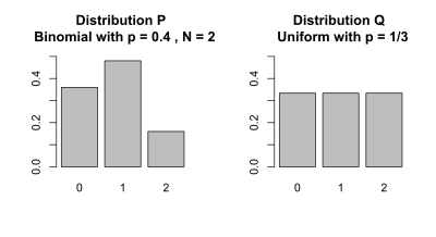
x	0	1	2
Distribution P(x)	0.36	0.48	0.16
Distribution Q(x)	0.333	0.333	0.333

The KL divergences $D_{\text{KL}}(P\parallel Q)$ and $D_{\text{KL}}(Q\parallel P)$ are calculated as follows. This example uses the natural log with base e, designated $\operatorname {ln}$ to get results in nats (see units of information).

{\begin{aligned}D_{\text{KL}}(P\parallel Q)&=\sum _{x\in {\mathcal {X}}}P(x)\ln \left({\frac {P(x)}{Q(x)}}\right)\\&=0.36\ln \left({\frac {0.36}{0.333}}\right)+0.48\ln \left({\frac {0.48}{0.333}}\right)+0.16\ln \left({\frac {0.16}{0.333}}\right)\\&=0.0852996\end{aligned}}

{\begin{aligned}D_{\text{KL}}(Q\parallel P)&=\sum _{x\in {\mathcal {X}}}Q(x)\ln \left({\frac {Q(x)}{P(x)}}\right)\\&=0.333\ln \left({\frac {0.333}{0.36}}\right)+0.333\ln \left({\frac {0.333}{0.48}}\right)+0.333\ln \left({\frac {0.333}{0.16}}\right)\\&=0.097455\end{aligned}}

Interpretations

The Kullback–Leibler divergence from $Q$ to $P$ is often denoted $D_{\text{KL}}(P\parallel Q)$ .

In the context of machine learning, $D_{\text{KL}}(P\parallel Q)$ is often called the information gain achieved if $Q$ is used instead of $P$ . By analogy with information theory, it is also called the relative entropy of $P$ with respect to $Q$ . In the context of coding theory, $D_{\text{KL}}(P\parallel Q)$ can be constructed by measuring the expected number of extra bits required to code samples from $P$ using a code optimized for $Q$ rather than the code optimized for $P$ .

Expressed in the language of Bayesian inference, $D_{\text{KL}}(P\parallel Q)$ is a measure of the information gained by revising one's beliefs from the prior probability distribution $Q$ to the posterior probability distribution $P$ . In other words, it is the amount of information lost when $Q$ is used to approximate $P$ .[6] In applications, $P$ typically represents the "true" distribution of data, observations, or a precisely calculated theoretical distribution, while $Q$ typically represents a theory, model, description, or approximation of $P$ . In order to find a distribution $Q$ that is closest to $P$ , we can minimize KL divergence and compute an information projection.

The Kullback–Leibler divergence is a special case of a broader class of statistical divergences called f-divergences as well as the class of Bregman divergences. It is the only such divergence over probabilities that is a member of both classes. Although it is often intuited as a way of measuring the distance between probability distributions, the Kullback–Leibler divergence is not a true metric. It does not obey the Triangle Inequality, and in general $D_{\text{KL}}(P\parallel Q)$ does not equal $D_{\text{KL}}(Q\parallel P)$ . However, its infinitesimal form, specifically its Hessian, gives a metric tensor known as the Fisher information metric.

Arthur Hobson proved that the Kullback–Leibler divergence is the only measure of difference between probability distributions that satisfies some desired properties, which are the canonical extension to those appearing in a commonly used characterization of entropy.[7] Consequently, mutual information is the only measure of mutual dependence that obeys certain related conditions, since it can be defined in terms of Kullback–Leibler divergence.

Motivation

Illustration of the Kullback–Leibler (KL) divergence for two normal distributions. The typical asymmetry for the Kullback–Leibler divergence is clearly visible.

In information theory, the Kraft–McMillan theorem establishes that any directly decodable coding scheme for coding a message to identify one value $x_{i}$ out of a set of possibilities $X$ can be seen as representing an implicit probability distribution $q(x_{i})=2^{-\ell _{i}}$ over $X$ , where $\ell _{i}$ is the length of the code for $x_{i}$ in bits. Therefore, the Kullback–Leibler divergence can be interpreted as the expected extra message-length per datum that must be communicated if a code that is optimal for a given (wrong) distribution $Q$ is used, compared to using a code based on the true distribution $P$ .

{\begin{aligned}D_{\text{KL}}(P\parallel Q)&=-\sum _{x\in {\mathcal {X}}}p(x)\log q(x)+\sum _{x\in {\mathcal {X}}}p(x)\log p(x)\\&=\mathrm {H} (P,Q)-\mathrm {H} (P)\end{aligned}}

where $\mathrm {H} (P,Q)$ is the cross entropy of $P$ and $Q$ , and $\mathrm {H} (P)$ is the entropy of $P$ (which is the same as the cross-entropy of P with itself).

The KL divergence $KL(P\parallel Q)$ can be thought of as something like a measurement of how far the distribution Q is from the distribution P. The cross-entropy $H(P,Q)$ is itself such a measurement, but it has the defect that $H(P,P)=:H(P)$ isn't zero, so we subtract $H(P)$ to make $KL(P\parallel Q)$ agree more closely with our notion of distance. (Unfortunately it still isn't symmetric.) There is a relation between the Kullback–Leibler divergence and the "rate function" in the theory of large deviations.[8][9]

Properties

The Kullback–Leibler divergence is always non-negative,

D_{\text{KL}}(P\parallel Q)\geq 0,

a result known as Gibbs' inequality, with

D_{\text{KL}}(P\parallel Q)

zero if and only if

P=Q

almost everywhere. The entropy

\mathrm {H} (P)

thus sets a minimum value for the cross-entropy

\mathrm {H} (P,Q)

, the expected number of bits required when using a code based on

Q

rather than

P

; and the Kullback–Leibler divergence therefore represents the expected number of extra bits that must be transmitted to identify a value

x

drawn from

X

, if a code is used corresponding to the probability distribution

Q

, rather than the "true" distribution

P

.

The Kullback–Leibler divergence remains well-defined for continuous distributions, and furthermore is invariant under parameter transformations. For example, if a transformation is made from variable $x$ to variable $y(x)$ , then, since $P(x)dx=P(y)dy$ and $Q(x)dx=Q(y)dy$ the Kullback–Leibler divergence may be rewritten:

{\begin{aligned}D_{\text{KL}}(P\parallel Q)&=\int _{x_{a}}^{x_{b}}P(x)\log \left({\frac {P(x)}{Q(x)}}\right)\,dx\\[6pt]&=\int _{y_{a}}^{y_{b}}P(y)\log \left({\frac {P(y)\,{\frac {dy}{dx}}}{Q(y)\,{\frac {dy}{dx}}}}\right)\,dy=\int _{y_{a}}^{y_{b}}P(y)\log \left({\frac {P(y)}{Q(y)}}\right)\,dy\end{aligned}}

where

y_{a}=y(x_{a})

and

y_{b}=y(x_{b})

. Although it was assumed that the transformation was continuous, this need not be the case. This also shows that the Kullback–Leibler divergence produces a dimensionally consistent quantity, since if

x

is a dimensioned variable,

P(x)

and

Q(x)

are also dimensioned, since e.g.

P(x)dx

is dimensionless. The argument of the logarithmic term is and remains dimensionless, as it must. It can therefore be seen as in some ways a more fundamental quantity than some other properties in information theory[10] (such as self-information or Shannon entropy), which can become undefined or negative for non-discrete probabilities.

The Kullback–Leibler divergence is additive for independent distributions in much the same way as Shannon entropy. If $P_{1},P_{2}$ are independent distributions, with the joint distribution $P(x,y)=P_{1}(x)P_{2}(y)$ , and $Q,Q_{1},Q_{2}$ likewise, then

D_{\text{KL}}(P\parallel Q)=D_{\text{KL}}(P_{1}\parallel Q_{1})+D_{\text{KL}}(P_{2}\parallel Q_{2}).

The Kullback–Leibler divergence $D_{\text{KL}}(P\parallel Q)$ is convex in the pair of probability mass functions $(p,q)$ , i.e. if $(p_{1},q_{1})$ and $(p_{2},q_{2})$ are two pairs of probability mass functions, then
$D_{\text{KL}}(\lambda p_{1}+(1-\lambda )p_{2}\parallel \lambda q_{1}+(1-\lambda )q_{2})\leq \lambda D_{\text{KL}}(p_{1}\parallel q_{1})+(1-\lambda )D_{\text{KL}}(p_{2}\parallel q_{2}){\text{ for }}0\leq \lambda \leq 1.$

Examples

Multivariate normal distributions

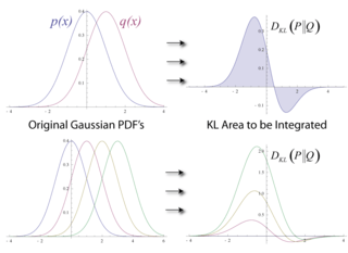
Suppose that we have two multivariate normal distributions, with means $\mu _{0},\mu _{1}$ and with (non-singular) covariance matrices $\Sigma _{0},\Sigma _{1}.$ If the two distributions have the same dimension, $k$ , then the Kullback–Leibler divergence between the distributions is as follows:[11]^{:p. 13}

D_{\text{KL}}\left({\mathcal {N}}_{0}\parallel {\mathcal {N}}_{1}\right)={\frac {1}{2}}\left(\operatorname {tr} \left(\Sigma _{1}^{-1}\Sigma _{0}\right)+\left(\mu _{1}-\mu _{0}\right)^{\mathsf {T}}\Sigma _{1}^{-1}\left(\mu _{1}-\mu _{0}\right)-k+\ln \left({\frac {\det \Sigma _{1}}{\det \Sigma _{0}}}\right)\right).

The logarithm in the last term must be taken to base e since all terms apart from the last are base-e logarithms of expressions that are either factors of the density function or otherwise arise naturally. The equation therefore gives a result measured in nats. Dividing the entire expression above by $\ln(2)$ yields the divergence in bits.

A special case, and a common quantity in variational inference, is the KL-divergence between a diagonal multivariate normal, and a standard normal distribution (with zero mean and unit variance):

D_{\text{KL}}\left({\mathcal {N}}\left(\left(\mu _{1},\ldots ,\mu _{k}\right)^{\mathsf {T}},\operatorname {diag} \left(\sigma _{1}^{2},\ldots ,\sigma _{k}^{2}\right)\right)\parallel {\mathcal {N}}\left(\mathbf {0} ,\mathbf {I} \right)\right)={1 \over 2}\sum _{i=1}^{k}\left(\sigma _{i}^{2}+\mu _{i}^{2}-1-\ln \left(\sigma _{i}^{2}\right)\right).

Relation to metrics

One might be tempted to call the Kullback–Leibler divergence a "distance metric" on the space of probability distributions, but this would not be correct as it is not symmetric – that is, $D_{\text{KL}}(P\parallel Q)\neq D_{\text{KL}}(Q\parallel P)$ – nor does it satisfy the triangle inequality. Even so, being a premetric, it generates a topology on the space of probability distributions. More concretely, if $\{P_{1},P_{2},\ldots \}$ is a sequence of distributions such that

\lim _{n\to \infty }D_{\text{KL}}(P_{n}\parallel Q)=0

then it is said that

P_{n}{\xrightarrow {D}}Q.

Pinsker's inequality entails that

P_{n}{\xrightarrow {D}}P\Rightarrow P_{n}{\xrightarrow {TV}}P,

where the latter stands for the usual convergence in total variation.

Fisher information metric

The Kullback–Leibler divergence is directly related to the Fisher information metric. This can be made explicit as follows. Assume that the probability distributions $P$ and $Q$ are both parameterized by some (possibly multi-dimensional) parameter $\theta$ . Consider then two close-by values of $P=P(\theta )$ and $Q=P(\theta _{0})$ so that the parameter $\theta$ differs by only a small amount from the parameter value $\theta _{0}$ . Specifically, up to first order one has (using the Einstein summation convention)

P(\theta )=P(\theta _{0})+\Delta \theta _{j}P_{j}(\theta _{0})+\cdots

with $\Delta \theta _{j}=(\theta -\theta _{0})_{j}$ a small change of $\theta$ in the $j$ direction, and $P_{j}\left(\theta _{0}\right)={\frac {\partial P}{\partial \theta _{j}}}(\theta _{0})$ the corresponding rate of change in the probability distribution. Since the Kullback–Leibler divergence has an absolute minimum 0 for $P=Q$ , i.e. $\theta =\theta _{0}$ , it changes only to second order in the small parameters $\Delta \theta _{j}$ . More formally, as for any minimum, the first derivatives of the divergence vanish

\left.{\frac {\partial }{\partial \theta _{j}}}\right|_{\theta =\theta _{0}}D_{\text{KL}}(P(\theta )\parallel P(\theta _{0}))=0,

and by the Taylor expansion one has up to second order

D_{\text{KL}}(P(\theta )\parallel P(\theta _{0}))={\frac {1}{2}}\Delta \theta _{j}\Delta \theta _{k}g_{jk}(\theta _{0})+\cdots

where the Hessian matrix of the divergence

g_{jk}(\theta _{0})=\left.{\frac {\partial ^{2}}{\partial \theta _{j}\,\partial \theta _{k}}}\right|_{\theta =\theta _{0}}D_{\text{KL}}(P(\theta )\parallel P(\theta _{0}))

must be positive semidefinite. Letting $\theta _{0}$ vary (and dropping the subindex 0) the Hessian $g_{jk}(\theta )$ defines a (possibly degenerate) Riemannian metric on the $θ$ parameter space, called the Fisher information metric.

Fisher information metric theorem

When $p_{(x,\rho )}$ satisfies the following regularity conditions:

{\tfrac {\partial \log(p)}{\partial \rho }},{\tfrac {\partial ^{2}\log(p)}{\partial \rho ^{2}}},{\tfrac {\partial ^{3}\log(p)}{\partial \rho ^{3}}}

exist,

{\begin{aligned}\left|{\frac {\partial p}{\partial \rho }}\right|&<F(x):\int _{x=0}^{\infty }F(x)\,dx<\infty ,\\\left|{\frac {\partial ^{2}p}{\partial \rho ^{2}}}\right|&<G(x):\int _{x=0}^{\infty }G(x)\,dx<\infty \\\left|{\frac {\partial ^{3}\log(p)}{\partial \rho ^{3}}}\right|&<H(x):\int _{x=0}^{\infty }p(x,0)H(x)\,dx<\xi <\infty \end{aligned}}

where $ξ$ is independent of $ρ$

\left.\int _{x=0}^{\infty }{\frac {\partial p(x,\rho )}{\partial \rho }}\right|_{\rho =0}\,dx=\left.\int _{x=0}^{\infty }{\frac {\partial ^{2}p(x,\rho )}{\partial \rho ^{2}}}\right|_{\rho =0}\,dx=0

then:

{\mathcal {D}}(p(x,0)\parallel p(x,\rho ))={\frac {c\rho ^{2}}{2}}+{\mathcal {O}}\left(\rho ^{3}\right){\text{ as }}\rho \to 0.

Variation of information

Another information-theoretic metric is Variation of information, which is roughly a symmetrization of conditional entropy. It is a metric on the set of partitions of a discrete probability space.

Relation to other quantities of information theory

Many of the other quantities of information theory can be interpreted as applications of the Kullback–Leibler divergence to specific cases.

Self-information

The self-information, also known as the information content of a signal, random variable, or event is defined as the negative logarithm of the probability of the given outcome occurring.

When applied to a discrete random variable, the self-information can be represented as

\operatorname {\operatorname {I} } (m)=D_{\text{KL}}\left(\delta _{\text{im}}\parallel \{p_{i}\}\right),

is the Kullback–Leibler divergence of the probability distribution $P(i)$ from a Kronecker delta representing certainty that $i=m$ — i.e. the number of extra bits that must be transmitted to identify $i$ if only the probability distribution $P(i)$ is available to the receiver, not the fact that $i=m$ .

Mutual information

The mutual information,

{\begin{aligned}\operatorname {I} (X;Y)&=D_{\text{KL}}(P(X,Y)\parallel P(X)P(Y))\\&=\operatorname {E} _{X}\{D_{\text{KL}}(P(Y\mid X)\parallel P(Y))\}\\&=\operatorname {E} _{Y}\{D_{\text{KL}}(P(X\mid Y)\parallel P(X))\}\end{aligned}}

is the Kullback–Leibler divergence of the product $P(X)P(Y)$ of the two marginal probability distributions from the joint probability distribution $P(X,Y)$ — i.e. the expected number of extra bits that must be transmitted to identify $X$ and $Y$ if they are coded using only their marginal distributions instead of the joint distribution. Equivalently, if the joint probability $P(X,Y)$ is known, it is the expected number of extra bits that must on average be sent to identify $Y$ if the value of $X$ is not already known to the receiver.

Shannon entropy

The Shannon entropy,

{\begin{aligned}\mathrm {H} (X)&=\operatorname {E} \left[\operatorname {I} _{X}(x)\right]\\&=\log(N)-D_{\text{KL}}\left(p_{X}(x)\parallel P_{U}(X)\right)\end{aligned}}

is the number of bits which would have to be transmitted to identify $X$ from $N$ equally likely possibilities, less the Kullback–Leibler divergence of the uniform distribution on the random variates of $X$ , $P_{U}(X)$ , from the true distribution $P(X)$ — i.e. less the expected number of bits saved, which would have had to be sent if the value of $X$ were coded according to the uniform distribution $P_{U}(X)$ rather than the true distribution $P(X)$ .

Conditional entropy

The conditional entropy,

{\begin{aligned}\mathrm {H} (X\mid Y)&=\log(N)-D_{\text{KL}}(P(X,Y)\parallel P_{U}(X)P(Y))\\&=\log(N)-D_{\text{KL}}(P(X,Y)\parallel P(X)P(Y))-D_{\text{KL}}(P(X)\parallel P_{U}(X))\\&=\mathrm {H} (X)-\operatorname {I} (X;Y)\\&=\log(N)-\operatorname {E} _{Y}\left[D_{\text{KL}}\left(P\left(X\mid Y\right)\parallel P_{U}(X)\right)\right]\end{aligned}}

is the number of bits which would have to be transmitted to identify $X$ from $N$ equally likely possibilities, less the Kullback–Leibler divergence of the product distribution $P_{U}(X)P(Y)$ from the true joint distribution $P(X,Y)$ — i.e. less the expected number of bits saved which would have had to be sent if the value of $X$ were coded according to the uniform distribution $P_{U}(X)$ rather than the conditional distribution $P(X|Y)$ of $X$ given $Y$ .

Cross entropy

When we have a set of possible events, coming from the distribution $p$ , we can encode them (with a lossless data compression) using entropy encoding. This compresses the data by replacing each fixed-length input symbol with a corresponding unique, variable-length, prefix-free code (e.g.: the events (A, B, C) with probabilities p = (1/2, 1/4, 1/4) can be encoded as the bits (0, 10, 11)). If we know the distribution $p$ in advance, we can devise an encoding that would be optimal (e.g.: using Huffman coding). Meaning the messages we encode will have the shortest length on average (assuming the encoded events are sampled from $p$ ), which will be equal to Shannon's Entropy of $p$ (denoted as $\mathrm {H} (p)$ ). However, if we use a different probability distribution ( $q$ ) when creating the entropy encoding scheme, then a larger number of bits will be needed to identify an event from a set of possibilities. This new (larger) number is measured by the cross entropy between $p$ and $q$ .

The cross entropy between two probability distributions ( $p$ and $q$ ) measures the average number of bits needed to identify an event from a set of possibilities, if a coding scheme is used based on a given probability distribution $q$ , rather than the "true" distribution $p$ . The cross entropy for two distributions $p$ and $q$ over the same probability space is thus defined as follows:

\mathrm {H} (p,q)=\operatorname {E} _{p}[-\log(q)]=\mathrm {H} (p)+D_{\text{KL}}(p\parallel q).

Under this scenario, the KL divergences can be interpreted as the extra number of bits, on average, that are needed (beyond $\mathrm {H} (p)$ ) for encoding the events because of using $q$ for constructing the encoding scheme instead of $p$ .

Bayesian updating

In Bayesian statistics the Kullback–Leibler divergence can be used as a measure of the information gain in moving from a prior distribution to a posterior distribution: $p(x)\to p(x\mid I)$ . If some new fact $Y=y$ is discovered, it can be used to update the posterior distribution for $X$ from $p(x\mid I)$ to a new posterior distribution $p(x\mid y,I)$ using Bayes' theorem:

p(x\mid y,I)={\frac {p(y\mid x,I)p(x\mid I)}{p(y\mid I)}}

This distribution has a new entropy:

\mathrm {H} {\big (}p(x\mid y,I){\big )}=-\sum _{x}p(x\mid y,I)\log p(x\mid y,I),

which may be less than or greater than the original entropy $\mathrm {H} (p(x\mid I))$ . However, from the standpoint of the new probability distribution one can estimate that to have used the original code based on $p(x\mid I)$ instead of a new code based on $p(x\mid y,I)$ would have added an expected number of bits:

D_{\text{KL}}{\big (}p(x\mid y,I)\parallel p(x\mid I){\big )}=\sum _{x}p(x\mid y,I)\log \left({\frac {p(x\mid y,I)}{p(x\mid I)}}\right)

to the message length. This therefore represents the amount of useful information, or information gain, about $X$ , that we can estimate has been learned by discovering $Y=y$ .

If a further piece of data, $Y_{2}=y_{2}$ , subsequently comes in, the probability distribution for $x$ can be updated further, to give a new best guess $p(x\mid y_{1},y_{2},I)$ . If one reinvestigates the information gain for using $p(x\mid y_{1},I)$ rather than $p(x\mid I)$ , it turns out that it may be either greater or less than previously estimated:

\sum _{x}p(x\mid y_{1},y_{2},I)\log \left({\frac {p(x\mid y_{1},y_{2},I)}{p(x\mid I)}}\right)

may be ≤ or > than

\displaystyle \sum _{x}p(x\mid y_{1},I)\log \left({\frac {p(x\mid y_{1},I)}{p(x\mid I)}}\right)

and so the combined information gain does not obey the triangle inequality:

D_{\text{KL}}{\big (}p(x\mid y_{1},y_{2},I)\parallel p(x\mid I){\big )}

may be <, = or > than

D_{\text{KL}}{\big (}p(x\mid y_{1},y_{2},I)\parallel p(x\mid y_{1},I){\big )}+D_{\text{KL}}{\big (}p(x\mid y_{1},I)\parallel p(x\mid I){\big )}

All one can say is that on average, averaging using $p(y_{2}\mid y_{1},x,I)$ , the two sides will average out.

Bayesian experimental design

A common goal in Bayesian experimental design is to maximise the expected Kullback–Leibler divergence between the prior and the posterior.[12] When posteriors are approximated to be Gaussian distributions, a design maximising the expected Kullback–Leibler divergence is called Bayes d-optimal.

Discrimination information

The Kullback–Leibler divergence ${\textstyle D_{\text{KL}}{\bigl (}p(x\mid H_{1})\parallel p(x\mid H_{0}){\bigr )}}$ can also be interpreted as the expected discrimination information for $H_{1}$ over $H_{0}$ : the mean information per sample for discriminating in favor of a hypothesis $H_{1}$ against a hypothesis $H_{0}$ , when hypothesis $H_{1}$ is true.[13] Another name for this quantity, given to it by I. J. Good, is the expected weight of evidence for $H_{1}$ over $H_{0}$ to be expected from each sample.

The expected weight of evidence for $H_{1}$ over $H_{0}$ is not the same as the information gain expected per sample about the probability distribution $p(H)$ of the hypotheses,

D_{\text{KL}}(p(x\mid H_{1})\parallel p(x\mid H_{0}))\neq IG=D_{\text{KL}}(p(H\mid x)\parallel p(H\mid I)).

Either of the two quantities can be used as a utility function in Bayesian experimental design, to choose an optimal next question to investigate: but they will in general lead to rather different experimental strategies.

On the entropy scale of information gain there is very little difference between near certainty and absolute certainty—coding according to a near certainty requires hardly any more bits than coding according to an absolute certainty. On the other hand, on the logit scale implied by weight of evidence, the difference between the two is enormous – infinite perhaps; this might reflect the difference between being almost sure (on a probabilistic level) that, say, the Riemann hypothesis is correct, compared to being certain that it is correct because one has a mathematical proof. These two different scales of loss function for uncertainty are both useful, according to how well each reflects the particular circumstances of the problem in question.

Principle of minimum discrimination information

The idea of Kullback–Leibler divergence as discrimination information led Kullback to propose the Principle of Minimum Discrimination Information (MDI): given new facts, a new distribution $f$ should be chosen which is as hard to discriminate from the original distribution $f_{0}$ as possible; so that the new data produces as small an information gain $D_{\text{KL}}(f\parallel f_{0})$ as possible.

For example, if one had a prior distribution $p(x,a)$ over $x$ and $a$ , and subsequently learnt the true distribution of $a$ was $u(a)$ , then the Kullback–Leibler divergence between the new joint distribution for $x$ and $a$ , $q(x\mid a)u(a)$ , and the earlier prior distribution would be:

D_{\text{KL}}(q(x\mid a)u(a)\parallel p(x,a))=\operatorname {E} _{u(a)}\left\{D_{\text{KL}}(q(x\mid a)\parallel p(x\mid a))\right\}+D_{\text{KL}}(u(a)\parallel p(a)),

i.e. the sum of the Kullback–Leibler divergence of $p(a)$ the prior distribution for $a$ from the updated distribution $u(a)$ , plus the expected value (using the probability distribution $u(a)$ ) of the Kullback–Leibler divergence of the prior conditional distribution $p(x\mid a)$ from the new conditional distribution $q(x\mid a)$ . (Note that often the later expected value is called the conditional Kullback–Leibler divergence (or conditional relative entropy) and denoted by $D_{\text{KL}}(q(x\mid a)\parallel p(x\mid a))$ [14]^{:p. 22}) This is minimized if $q(x\mid a)=p(x\mid a)$ over the whole support of $u(a)$ ; and we note that this result incorporates Bayes' theorem, if the new distribution $u(a)$ is in fact a δ function representing certainty that $a$ has one particular value.

MDI can be seen as an extension of Laplace's Principle of Insufficient Reason, and the Principle of Maximum Entropy of E.T. Jaynes. In particular, it is the natural extension of the principle of maximum entropy from discrete to continuous distributions, for which Shannon entropy ceases to be so useful (see differential entropy), but the Kullback–Leibler divergence continues to be just as relevant.

In the engineering literature, MDI is sometimes called the Principle of Minimum Cross-Entropy (MCE) or Minxent for short. Minimising the Kullback–Leibler divergence from $m$ to $p$ with respect to $m$ is equivalent to minimizing the cross-entropy of $p$ and $m$ , since

\mathrm {H} (p,m)=\mathrm {H} (p)+D_{\text{KL}}(p\parallel m),

which is appropriate if one is trying to choose an adequate approximation to $p$ . However, this is just as often not the task one is trying to achieve. Instead, just as often it is $m$ that is some fixed prior reference measure, and $p$ that one is attempting to optimise by minimising $D_{\text{KL}}(p\parallel m)$ subject to some constraint. This has led to some ambiguity in the literature, with some authors attempting to resolve the inconsistency by redefining cross-entropy to be $D_{\text{KL}}(p\parallel m)$ , rather than $\mathrm {H} (p,m)$ .

Relationship to available work

Pressure versus volume plot of available work from a mole of argon gas relative to ambient, calculated as

T_{o}

times the Kullback–Leibler divergence.

Surprisals[15] add where probabilities multiply. The surprisal for an event of probability $p$ is defined as $s=k\ln(1/p)$ . If $k$ is $\left\{1,1/\ln 2,1.38\times 10^{-23}\right\}$ then surprisal is in $\{$ nats, bits, or $J/K\}$ so that, for instance, there are $N$ bits of surprisal for landing all "heads" on a toss of $N$ coins.

Best-guess states (e.g. for atoms in a gas) are inferred by maximizing the average surprisal $S$ (entropy) for a given set of control parameters (like pressure $P$ or volume $V$ ). This constrained entropy maximization, both classically[16] and quantum mechanically,[17] minimizes Gibbs availability in entropy units[18] $A\equiv -k\ln(Z)$ where $Z$ is a constrained multiplicity or partition function.

When temperature $T$ is fixed, free energy ( $T\times A$ ) is also minimized. Thus if $T,V$ and number of molecules $N$ are constant, the Helmholtz free energy $F\equiv U-TS$ (where $U$ is energy) is minimized as a system "equilibrates." If $T$ and $P$ are held constant (say during processes in your body), the Gibbs free energy $G=U+PV-TS$ is minimized instead. The change in free energy under these conditions is a measure of available work that might be done in the process. Thus available work for an ideal gas at constant temperature $T_{o}$ and pressure $P_{o}$ is $W=\Delta G=NkT_{o}\Theta (V/V_{o})$ where $V_{o}=NkT_{o}/P_{o}$ and $\Theta (x)=x-1-\ln x\geq 0$ (see also Gibbs inequality).

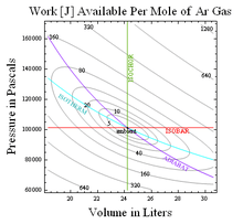
More generally[19] the work available relative to some ambient is obtained by multiplying ambient temperature $T_{o}$ by Kullback–Leibler divergence or net surprisal $\Delta I\geq 0,$ defined as the average value of $k\ln(p/p_{o})$ where $p_{o}$ is the probability of a given state under ambient conditions. For instance, the work available in equilibrating a monatomic ideal gas to ambient values of $V_{o}$ and $T_{o}$ is thus $W=T_{o}\Delta I$ , where Kullback–Leibler divergence

\Delta I=Nk\left[\Theta \left({\frac {V}{V_{o}}}\right)+{\frac {3}{2}}\Theta \left({\frac {T}{T_{o}}}\right)\right].

The resulting contours of constant Kullback–Leibler divergence, shown at right for a mole of Argon at standard temperature and pressure, for example put limits on the conversion of hot to cold as in flame-powered air-conditioning or in the unpowered device to convert boiling-water to ice-water discussed here.[20] Thus Kullback–Leibler divergence measures thermodynamic availability in bits.

Quantum information theory

For density matrices $P$ and $Q$ on a Hilbert space, the K–L divergence (or quantum relative entropy as it is often called in this case) from $Q$ to $P$ is defined to be

D_{\text{KL}}(P\parallel Q)=\operatorname {Tr} (P(\log(P)-\log(Q))).

In quantum information science the minimum of $D_{\text{KL}}(P\parallel Q)$ over all separable states $Q$ can also be used as a measure of entanglement in the state $P$ .

Relationship between models and reality

Just as Kullback–Leibler divergence of "actual from ambient" measures thermodynamic availability, Kullback–Leibler divergence of "reality from a model" is also useful even if the only clues we have about reality are some experimental measurements. In the former case Kullback–Leibler divergence describes distance to equilibrium or (when multiplied by ambient temperature) the amount of available work, while in the latter case it tells you about surprises that reality has up its sleeve or, in other words, how much the model has yet to learn.

Although this tool for evaluating models against systems that are accessible experimentally may be applied in any field, its application to selecting a statistical model via Akaike information criterion are particularly well described in papers[21] and a book[22] by Burnham and Anderson. In a nutshell the Kullback–Leibler divergence of reality from a model may be estimated, to within a constant additive term, by a function (like the squares summed) of the deviations observed between data and the model's predictions. Estimates of such divergence for models that share the same additive term can in turn be used to select among models.

When trying to fit parametrized models to data there are various estimators which attempt to minimize Kullback–Leibler divergence, such as maximum likelihood and maximum spacing estimators.

Symmetrised divergence

Kullback and Leibler themselves actually defined the divergence as:

D_{\text{KL}}(P\parallel Q)+D_{\text{KL}}(Q\parallel P)

which is symmetric and nonnegative. This quantity has sometimes been used for feature selection in classification problems, where $P$ and $Q$ are the conditional pdfs of a feature under two different classes. In the Banking and Finance industries, this quantity is referred to as Population Stability Index, and is used to assess distributional shifts in model features through time.

An alternative is given via the $\lambda$ divergence,

D_{\lambda }(P\parallel Q)=\lambda D_{\text{KL}}(P\parallel \lambda P+(1-\lambda )Q)+(1-\lambda )D_{\text{KL}}(Q\parallel \lambda P+(1-\lambda )Q),

which can be interpreted as the expected information gain about $X$ from discovering which probability distribution $X$ is drawn from, $P$ or $Q$ , if they currently have probabilities $\lambda$ and $1-\lambda$ respectively.

The value $\lambda =0.5$ gives the Jensen–Shannon divergence, defined by

D_{\text{JS}}={\frac {1}{2}}D_{\text{KL}}(P\parallel M)+{\frac {1}{2}}D_{\text{KL}}(Q\parallel M)

where $M$ is the average of the two distributions,

M={\frac {1}{2}}(P+Q).

$D_{JS}$ can also be interpreted as the capacity of a noisy information channel with two inputs giving the output distributions $P$ and $Q$ . The Jensen–Shannon divergence, like all f-divergences, is locally proportional to the Fisher information metric. It is similar to the Hellinger metric (in the sense that induces the same affine connection on a statistical manifold).

Relationship to other probability-distance measures

There are many other important measures of probability distance. Some of these are particularly connected with the Kullback–Leibler divergence. For example:

The total variation distance, $\delta (p,q)$ . This is connected to the divergence through Pinsker's inequality: $\delta (P,Q)\leq {\sqrt {{\frac {1}{2}}D_{\text{KL}}(P\parallel Q)}}$
The family of Rényi divergences provide generalizations of the Kullback–Leibler divergence. Depending on the value of a certain parameter, $\alpha$ , various inequalities may be deduced.

Other notable measures of distance include the Hellinger distance, histogram intersection, Chi-squared statistic, quadratic form distance, match distance, Kolmogorov–Smirnov distance, and earth mover's distance.[23]

Data differencing

Just as absolute entropy serves as theoretical background for data compression, relative entropy serves as theoretical background for data differencing – the absolute entropy of a set of data in this sense being the data required to reconstruct it (minimum compressed size), while the relative entropy of a target set of data, given a source set of data, is the data required to reconstruct the target given the source (minimum size of a patch).

References

Kullback, S.; Leibler, R.A. (1951). "On information and sufficiency". Annals of Mathematical Statistics. 22 (1): 79–86. doi:10.1214/aoms/1177729694. JSTOR 2236703. MR 0039968.
Kullback, S. (1959), Information Theory and Statistics, John Wiley & Sons. Republished by Dover Publications in 1968; reprinted in 1978: ISBN 0-8446-5625-9.
Kullback, S. (1987). "Letter to the Editor: The Kullback–Leibler distance". The American Statistician. 41 (4): 340–341. doi:10.1080/00031305.1987.10475510. JSTOR 2684769.
MacKay, David J.C. (2003). Information Theory, Inference, and Learning Algorithms (First ed.). Cambridge University Press. p. 34. ISBN 9780521642989.
Bishop C. (2006). Pattern Recognition and Machine Learning
Burnham, K. P.; Anderson, D. R. (2002). Model Selection and Multi-Model Inference (2nd ed.). Springer. p. 51. ISBN 9780387953649.
Hobson, Arthur (1971). Concepts in statistical mechanics. New York: Gordon and Breach. ISBN 978-0677032405.
Sanov, I.N. (1957). "On the probability of large deviations of random magnitudes". Mat. Sbornik. 42 (84): 11–44.
Novak S.Y. (2011), Extreme Value Methods with Applications to Finance ch. 14.5 (Chapman & Hall). ISBN 978-1-4398-3574-6.
See the section "differential entropy – 4" in Relative Entropy video lecture by Sergio Verdú NIPS 2009
Duchi J., "Derivations for Linear Algebra and Optimization".
Chaloner, K.; Verdinelli, I. (1995). "Bayesian experimental design: a review". Statistical Science. 10 (3): 273–304. doi:10.1214/ss/1177009939.
Press, W.H.; Teukolsky, S.A.; Vetterling, W.T.; Flannery, B.P. (2007). "Section 14.7.2. Kullback–Leibler Distance". Numerical Recipes: The Art of Scientific Computing (3rd ed.). Cambridge University Press. ISBN 978-0-521-88068-8.
Thomas M. Cover, Joy A. Thomas (1991) Elements of Information Theory (John Wiley & Sons)
Myron Tribus (1961), Thermodynamics and Thermostatics (D. Van Nostrand, New York)
Jaynes, E. T. (1957). "Information theory and statistical mechanics" (PDF). Physical Review. 106 (4): 620–630. Bibcode:1957PhRv..106..620J. doi:10.1103/physrev.106.620.
Jaynes, E. T. (1957). "Information theory and statistical mechanics II" (PDF). Physical Review. 108 (2): 171–190. Bibcode:1957PhRv..108..171J. doi:10.1103/physrev.108.171.
J.W. Gibbs (1873), "A method of geometrical representation of thermodynamic properties of substances by means of surfaces", reprinted in The Collected Works of J. W. Gibbs, Volume I Thermodynamics, ed. W. R. Longley and R. G. Van Name (New York: Longmans, Green, 1931) footnote page 52.
Tribus, M.; McIrvine, E. C. (1971). "Energy and information". Scientific American. 224 (3): 179–186. Bibcode:1971SciAm.225c.179T. doi:10.1038/scientificamerican0971-179.
Fraundorf, P. (2007). "Thermal roots of correlation-based complexity". Complexity. 13 (3): 18–26. arXiv:1103.2481. Bibcode:2008Cmplx..13c..18F. doi:10.1002/cplx.20195.
Burnham, K.P.; Anderson, D.R. (2001). "Kullback–Leibler information as a basis for strong inference in ecological studies". Wildlife Research. 28 (2): 111–119. doi:10.1071/WR99107.
Burnham, K. P. and Anderson D. R. (2002), Model Selection and Multimodel Inference: A Practical Information-Theoretic Approach, Second Edition (Springer Science) ISBN 978-0-387-95364-9.
Rubner, Y.; Tomasi, C.; Guibas, L. J. (2000). "The earth mover's distance as a metric for image retrieval". International Journal of Computer Vision. 40 (2): 99–121. doi:10.1023/A:1026543900054.

External links

This article is issued from Wikipedia. The text is licensed under Creative Commons - Attribution - Sharealike. Additional terms may apply for the media files.

[1] Kullback, S.; Leibler, R.A. (1951). "On information and sufficiency". Annals of Mathematical Statistics. 22 (1): 79–86. doi:10.1214/aoms/1177729694. JSTOR 2236703. MR 0039968.

[Kullback-2] Kullback, S. (1959), Information Theory and Statistics, John Wiley & Sons. Republished by Dover Publications in 1968; reprinted in 1978: ISBN 0-8446-5625-9.

[3] Kullback, S. (1987). "Letter to the Editor: The Kullback–Leibler distance". The American Statistician. 41 (4): 340–341. doi:10.1080/00031305.1987.10475510. JSTOR 2684769.

[4] MacKay, David J.C. (2003). Information Theory, Inference, and Learning Algorithms (First ed.). Cambridge University Press. p. 34. ISBN 9780521642989.

[5] Bishop C. (2006). Pattern Recognition and Machine Learning

[6] Burnham, K. P.; Anderson, D. R. (2002). Model Selection and Multi-Model Inference (2nd ed.). Springer. p. 51. ISBN 9780387953649.

[7] Hobson, Arthur (1971). Concepts in statistical mechanics. New York: Gordon and Breach. ISBN 978-0677032405.

[Sanov-8] Sanov, I.N. (1957). "On the probability of large deviations of random magnitudes". Mat. Sbornik. 42 (84): 11–44.

[Novak-9] Novak S.Y. (2011), Extreme Value Methods with Applications to Finance ch. 14.5 (Chapman & Hall). ISBN 978-1-4398-3574-6.

[VerduLecture-10] See the section "differential entropy – 4" in Relative Entropy video lecture by Sergio Verdú NIPS 2009

[11] Duchi J., "Derivations for Linear Algebra and Optimization".

[12] Chaloner, K.; Verdinelli, I. (1995). "Bayesian experimental design: a review". Statistical Science. 10 (3): 273–304. doi:10.1214/ss/1177009939.

[13] Press, W.H.; Teukolsky, S.A.; Vetterling, W.T.; Flannery, B.P. (2007). "Section 14.7.2. Kullback–Leibler Distance". Numerical Recipes: The Art of Scientific Computing (3rd ed.). Cambridge University Press. ISBN 978-0-521-88068-8.

[14] Thomas M. Cover, Joy A. Thomas (1991) Elements of Information Theory (John Wiley & Sons)

[15] Myron Tribus (1961), Thermodynamics and Thermostatics (D. Van Nostrand, New York)

[16] Jaynes, E. T. (1957). "Information theory and statistical mechanics" (PDF). Physical Review. 106 (4): 620–630. Bibcode:1957PhRv..106..620J. doi:10.1103/physrev.106.620.

[17] Jaynes, E. T. (1957). "Information theory and statistical mechanics II" (PDF). Physical Review. 108 (2): 171–190. Bibcode:1957PhRv..108..171J. doi:10.1103/physrev.108.171.

[18] J.W. Gibbs (1873), "A method of geometrical representation of thermodynamic properties of substances by means of surfaces", reprinted in The Collected Works of J. W. Gibbs, Volume I Thermodynamics, ed. W. R. Longley and R. G. Van Name (New York: Longmans, Green, 1931) footnote page 52.

[19] Tribus, M.; McIrvine, E. C. (1971). "Energy and information". Scientific American. 224 (3): 179–186. Bibcode:1971SciAm.225c.179T. doi:10.1038/scientificamerican0971-179.

[20] Fraundorf, P. (2007). "Thermal roots of correlation-based complexity". Complexity. 13 (3): 18–26. arXiv:1103.2481. Bibcode:2008Cmplx..13c..18F. doi:10.1002/cplx.20195.

[21] Burnham, K.P.; Anderson, D.R. (2001). "Kullback–Leibler information as a basis for strong inference in ecological studies". Wildlife Research. 28 (2): 111–119. doi:10.1071/WR99107.

[22] Burnham, K. P. and Anderson D. R. (2002), Model Selection and Multimodel Inference: A Practical Information-Theoretic Approach, Second Edition (Springer Science) ISBN 978-0-387-95364-9.

[earth-23] Rubner, Y.; Tomasi, C.; Guibas, L. J. (2000). "The earth mover's distance as a metric for image retrieval". International Journal of Computer Vision. 40 (2): 99–121. doi:10.1023/A:1026543900054.