Kelvin–Stokes theorem

The Kelvin–Stokes theorem,[1][2] named after Lord Kelvin and George Stokes, also known as the Stokes' theorem,[3] the fundamental theorem for curls or simply the curl theorem,[4] is a theorem in vector calculus on $\mathbb {R} ^{3}$ . Given a vector field, the theorem relates the integral of the curl of the vector field over some surface, to the line integral of the vector field around the boundary of the surface.

An illustration of the Kelvin–Stokes theorem, with surface

Σ

, its boundary

\partialΣ

and the normal vector

n

.

If a vector field $\mathbf {A} =(P(x,y,z),Q(x,y,z),R(x,y,z))$ is defined in a region with smooth oriented surface $\Sigma$ and has first order continuous partial derivatives then:

{\begin{aligned}\iint \limits _{\Sigma }(\nabla \times \mathbf {A} )\cdot d\mathbf {a} &=\iint \limits _{\Sigma }{\Bigg (}\left({\frac {\partial R}{\partial y}}-{\frac {\partial Q}{\partial z}}\right)\,dy\,dz+\left({\frac {\partial P}{\partial z}}-{\frac {\partial R}{\partial x}}\right)\,dz\,dx+\left({\frac {\partial Q}{\partial x}}-{\frac {\partial P}{\partial y}}\right)\,dx\,dy{\Bigg )}\\&=\oint \limits _{\partial \Sigma }{\Big (}P\,dx+Q\,dy+R\,dz{\Big )}=\oint \limits _{\partial \Sigma }\mathbf {A} \cdot d\mathbf {l} ,\end{aligned}}

where $\partial \Sigma$ is boundary of region with smooth surface $\Sigma$ .

The above classical Kelvin-Stokes theorem can be stated in one sentence: The line integral of a vector field over a loop is equal to the flux of its curl through the enclosed surface.

The Kelvin–Stokes theorem is a special case of the "generalized Stokes' theorem."[5][6] In particular, a vector field on $\mathbb {R} ^{3}$ can be considered as a 1-form in which case its curl is its exterior derivative, a 2-form.

Theorem

The main challenge in a precise statement of Stokes' theorem is in defining the notion of a boundary. Surfaces such as the Koch snowflake, for example, are well-known not to exhibit a Riemann-integrable boundary, and the notion of surface measure in Lebesgue theory cannot be defined for a non-Lipschitz surface. One (advanced) technique is to pass to a weak formulation and then apply the machinery of geometric measure theory; for that approach see the coarea formula. In this article, we instead use a more elementary definition, based on the fact that a boundary can be discerned for full-dimensional subsets of $ℝ 2$ .

Let $γ : [a, b] \to R 2$ be a piecewise smooth Jordan plane curve. The Jordan curve theorem implies that $γ$ divides $R 2$ into two components, a compact one and another that is non-compact. Let $D$ denote the compact part; then $D$ is bounded by $γ$ . It now suffices to transfer this notion of boundary along a continuous map to our surface in $ℝ 3$ . But we already have such a map: the parametrization of $Σ$ .

Suppose $ψ : D \to R 3$ is smooth, with $Σ = ψ (D)$ . If $Γ$ is the space curve defined by $Γ (t) = ψ (γ (t))$ [note 1], then we call $Γ$ the boundary of $Σ$ , written $\partial Σ$ .

With the above notation, if $F$ is any smooth vector field on $R 3$ , then[7][8]

\oint _{\partial \Sigma }\mathbf {F} \,\cdot \,d{\mathbf {\Gamma } }=\iint _{\Sigma }\nabla \times \mathbf {F} \,\cdot \,d\mathbf {S} .

Proof

The proof of the theorem consists of 4 steps. We assume Green's theorem, so what is of concern is how to boil down the three-dimensional complicated problem (Kelvin–Stokes theorem) to a two-dimensional rudimentary problem (Green's theorem).[9] When proving this theorem, mathematicians normally deduce it as a special case of a more general result, which is stated in terms of differential forms, and proved using more sophisticated machinery. While powerful, these techniques require substantial background, so the proof below avoids them, and does not presuppose any knowledge beyond a familiarity with basic vector calculus.[8] At the end of this section, a short alternate proof of the Kelvin-Stokes theorem is given, as a corollary of the generalized Stokes' Theorem.

Elementary proof

First step of the proof (parametrization of integral)

As in Theorem § Notes, we reduce the dimension by using the natural parametrization of the surface. Let $ψ$ and $γ$ be as in that section, and note that by change of variables

\oint _{\partial \Sigma }{\mathbf {F} (\mathbf {x} )\cdot \,d\mathbf {l} }=\oint _{\gamma }{\mathbf {F} (\mathbf {\psi } (\mathbf {y} ))\cdot \,d\mathbf {\psi } (\mathbf {y} )}=\oint _{\gamma }{\mathbf {F} (\mathbf {\psi } (\mathbf {y} ))J_{\mathbf {y} }(\mathbf {\psi } )\,d\mathbf {y} }

where $Jψ$ stands for the Jacobian matrix of $ψ$ .

Now let ${e u, e v}$ be an orthonormal basis in the coordinate directions of $ℝ 2$ . Recognizing that the columns of $J y ψ$ are precisely the partial derivatives of $ψ$ at $y$ , we can expand the previous equation in coordinates as

{\begin{aligned}\oint _{\partial \Sigma }{\mathbf {F} (\mathbf {x} )\cdot \,d\mathbf {l} }&=\oint _{\gamma }{\mathbf {F} (\mathbf {\psi } (\mathbf {y} ))J_{\mathbf {y} }(\mathbf {\psi } )\mathbf {e} _{u}(\mathbf {e} _{u}\cdot \,d\mathbf {y} )+\mathbf {F} (\mathbf {\psi } (\mathbf {y} ))J_{\mathbf {y} }(\mathbf {\psi } )\mathbf {e} _{v}(\mathbf {e} _{v}\cdot \,d\mathbf {y} )}\\&=\oint _{\gamma }{\left(\left(\mathbf {F} (\mathbf {\psi } (\mathbf {y} ))\cdot {\frac {\partial \mathbf {\psi } }{\partial u}}(\mathbf {y} )\right)\mathbf {e} _{u}+\left(\mathbf {F} (\mathbf {\psi } (\mathbf {y} ))\cdot {\frac {\partial \mathbf {\psi } }{\partial v}}(\mathbf {y} )\right)\mathbf {e} _{v}\right)\cdot \,d\mathbf {y} }\end{aligned}}

Second step in the proof (defining the pullback)

The previous step suggests we define the function

\mathbf {P} (u,v)=\left(\mathbf {F} (\mathbf {\psi } (u,v))\cdot {\frac {\partial \mathbf {\psi } }{\partial u}}(u,v)\right)\mathbf {e} _{u}+\left(\mathbf {F} (\mathbf {\psi } (u,v))\cdot {\frac {\partial \mathbf {\psi } }{\partial v}}\right)\mathbf {e} _{v}

This is the pullback of $F$ along $ψ$ , and, by the above, it satisfies

\oint _{\partial \Sigma }{\mathbf {F} (\mathbf {x} )\cdot \,d\mathbf {l} }=\oint _{\gamma }{\mathbf {P} (\mathbf {y} )\cdot \,d\mathbf {l} }

We have successfully reduced one side of Stokes' theorem to a 2-dimensional formula; we now turn to the other side.

Third step of the proof (second equation)

First, calculate the partial derivatives appearing in Green's theorem, via the product rule:

{\begin{aligned}{\frac {\partial P_{1}}{\partial v}}&={\frac {\partial (\mathbf {F} \circ \psi )}{\partial v}}\cdot {\frac {\partial \psi }{\partial u}}+(\mathbf {F} \circ \psi )\cdot {\frac {\partial ^{2}\psi }{\partial v\partial u}}\\{\frac {\partial P_{2}}{\partial u}}&={\frac {\partial (\mathbf {F} \circ \psi )}{\partial u}}\cdot {\frac {\partial \psi }{\partial v}}+(\mathbf {F} \circ \psi )\cdot {\frac {\partial ^{2}\psi }{\partial u\partial v}}\end{aligned}}

Conveniently, the second term vanishes in the difference, by equality of mixed partials. So,

{\begin{aligned}{\frac {\partial P_{1}}{\partial v}}-{\frac {\partial P_{2}}{\partial u}}&={\frac {\partial (\mathbf {F} \circ \psi )}{\partial v}}\cdot {\frac {\partial \psi }{\partial u}}-{\frac {\partial (\mathbf {F} \circ \psi )}{\partial u}}\cdot {\frac {\partial \psi }{\partial v}}\\&={\frac {\partial \psi }{\partial u}}(J_{\psi (u,v)}\mathbf {F} ){\frac {\partial \psi }{\partial v}}-{\frac {\partial \psi }{\partial v}}(J_{\psi (u,v)}\mathbf {F} ){\frac {\partial \psi }{\partial u}}&&{\text{ (chain rule)}}\\&={\frac {\partial \psi }{\partial u}}(J_{\psi (u,v)}\mathbf {F} -(J_{\psi (u,v)}\mathbf {F} )^{\mathsf {T}}){\frac {\partial \psi }{\partial v}}\end{aligned}}

But now consider the matrix in that quadratic form—that is, $J_{\psi (u,v)}\mathbf {F} -(J_{\psi (u,v)}\mathbf {F} )^{\mathsf {T}}$ . We claim this matrix in fact describes a cross product.

To be precise, let $A=(A_{ij})_{ij}$ be an arbitrary $3 \times 3$ matrix and let

\mathbf {a} ={\begin{pmatrix}A_{32}-A_{23}\\A_{13}-A_{31}\\A_{21}-A_{12}\end{pmatrix}}

Note that $x \mapsto a \times x$ is linear, so it is determined by its action on basis elements. But by direct calculation

{\begin{aligned}(A-A^{\mathsf {T}})\mathbf {e} _{1}&={\begin{pmatrix}0\\a_{3}\\-a_{2}\end{pmatrix}}=\mathbf {a} \times \mathbf {e} _{1}\\(A-A^{\mathsf {T}})\mathbf {e} _{2}&={\begin{pmatrix}-a_{3}\\0\\a_{1}\end{pmatrix}}=\mathbf {a} \times \mathbf {e} _{2}\\(A-A^{\mathsf {T}})\mathbf {e} _{3}&={\begin{pmatrix}a_{2}\\-a_{1}\\0\end{pmatrix}}=\mathbf {a} \times \mathbf {e} _{3}\end{aligned}}

Thus $(A - A T) x = a \times x$ for any $x$ . Substituting $J F$ for $A$ , we obtain

({(J_{\psi (u,v)}\mathbf {F} )}_{\psi (u,v)}-{(J_{\psi (u,v)}\mathbf {F} )}^{\mathsf {T}})\mathbf {x} =(\nabla \times \mathbf {F} )\times \mathbf {x} ,\quad {\text{for all}}\,\mathbf {x} \in \mathbf {R} ^{3}

We can now recognize the difference of partials as a (scalar) triple product:

{\begin{aligned}{\frac {\partial P_{1}}{\partial v}}-{\frac {\partial P_{2}}{\partial u}}&={\frac {\partial \psi }{\partial u}}\cdot (\nabla \times \mathbf {F} )\times {\frac {\partial \psi }{\partial v}}\\&=\det \left[(\nabla \times \mathbf {F} )(\psi (u,v))\quad {\frac {\partial \psi }{\partial u}}(u,v)\quad {\frac {\partial \psi }{\partial v}}(u,v)\right]\end{aligned}}

On the other hand, the definition of a surface integral also includes a triple product—the very same one!

{\begin{aligned}\iint _{S}(\nabla \times \mathbf {F} )\cdot \,d^{2}\mathbf {S} &=\iint _{D}{(\nabla \times \mathbf {F} )(\psi (u,v))\cdot \left({\frac {\partial \psi }{\partial u}}(u,v)\times {\frac {\partial \psi }{\partial v}}(u,v)\,du\,dv\right)}\\&=\iint _{D}\det \left[(\nabla \times \mathbf {F} )(\psi (u,v))\quad {\frac {\partial \psi }{\partial u}}(u,v)\quad {\frac {\partial \psi }{\partial v}}(u,v)\right]\,du\,dv\end{aligned}}

So, we obtain

\iint _{S}(\nabla \times \mathbf {F} )\cdot \,d^{2}\mathbf {S} =\iint _{D}\left({\frac {\partial P_{2}}{\partial u}}-{\frac {\partial P_{1}}{\partial v}}\right)\,du\,dv

Fourth step of the proof (reduction to Green's theorem)

Combining the second and third steps, and then applying Green's theorem completes the proof.

Proof via differential forms

$ℝ \to ℝ 3$ can be identified with the differential 1-forms on $ℝ 3$ via the map

F_{1}\mathbf {e} _{1}+F_{2}\mathbf {e} _{2}+F_{3}\mathbf {e} _{3}\mapsto F_{1}\,dx+F_{2}\,dy+F_{3}dy

.

Write the differential 1-form associated to a function $F$ as $ω F$ . Then one can calculate that

\star \omega _{\nabla \times \mathbf {F} }=d\omega _{\mathbf {F} }

where $★$ is the Hodge star and $d$ is the exterior derivative. Thus, by generalized Stokes' theorem,[10]

\oint _{\partial \Sigma }{\mathbf {F} \cdot \,d\mathbf {l} }=\oint _{\partial \Sigma }{\omega _{\mathbf {F} }}=\int _{\Sigma }{d\omega _{\mathbf {F} }}=\int _{\Sigma }{\star \omega _{\nabla \times \mathbf {F} }}=\iint _{\Sigma }{\nabla \times \mathbf {F} \cdot \,d^{2}\mathbf {S} }

Applications

In fluid dynamics

In this section, we will discuss the lamellar vector field based on Kelvin–Stokes theorem.

Irrotational fields

Definition 2-1 (Irrotational field). A smooth vector field $F$ on an open $U \subseteq R 3$ is irrotational if $\nabla \times F = 0$ .

If the domain of F is simply connected, then $F$ is a conservative vector field.

Helmholtz's theorems

In this section, we will introduce a theorem that is derived from the Kelvin–Stokes theorem and characterizes vortex-free vector fields. In fluid dynamics it is called Helmholtz's theorems.

Theorem 2-1 (Helmholtz's Theorem in Fluid Dynamics).[5][2]^:142 Let $U \subseteq R 3$ be an open subset with a lamellar vector field $F$ and let $c 0, c 1 : [0, 1] \to U$ be piecewise smooth loops. If there is a function $H : [0, 1] \times [0, 1] \to U$ such that

[TLH0] $H$ is piecewise smooth,
[TLH1] $H (t, 0) = c 0 (t)$ for all $t \in [0, 1]$ ,
[TLH2] $H (t, 1) = c 1 (t)$ for all $t \in [0, 1]$ ,
[TLH3] $H (0, s) = H (1, s)$ for all $s \in [0, 1]$ .

Then,

\int _{c_{0}}\mathbf {F} \,dc_{0}=\int _{c_{1}}\mathbf {F} \,dc_{1}

Some textbooks such as Lawrence[5] call the relationship between $c 0$ and $c 1$ stated in Theorem 2-1 as "homotopic" and the function $H : [0, 1] \times [0, 1] \to U$ as "homotopy between $c 0$ and $c 1$ ". However, "homotopic" or "homotopy" in above-mentioned sense are different (stronger than) typical definitions of "homotopic" or "homotopy"; the latter omit condition [TLH3]. So from now on we refer to homotopy (homotope) in the sense of Theorem 2-1 as a tubular homotopy (resp. tubular-homotopic).[note 2]

Proof of the theorem

The definitions of

γ 1, ..., γ 4

In what follows, we abuse notation and use " $+$ " for concatenation of paths in the fundamental groupoid and " $-$ " for reversing the orientation of a path.

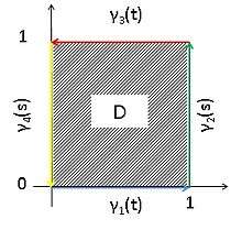
Let $D = [0, 1] \times [0, 1]$ , and split $\partial D$ into 4 line segments $γ j$ .

{\begin{aligned}\gamma _{1}:[0,1]\to D;\quad &\gamma _{1}(t)=(t,0)\\\gamma _{2}:[0,1]\to D;\quad &\gamma _{2}(s)=(1,s)\\\gamma _{3}:[0,1]\to D;\quad &\gamma _{3}(t)=(1-t,1)\\\gamma _{4}:[0,1]\to D;\quad &\gamma _{4}(s)=(0,1-s)\partial D=\gamma _{1}+\gamma _{2}+\gamma _{3}+\gamma _{4}\end{aligned}}

By our assumption that $c 1$ and $c 2$ are piecewise smooth homotopic, there is a piecewise smooth homotopy $H : D \to M$

{\begin{aligned}\Gamma _{i}(t)&=H(\gamma _{i}(t))&&i=1,2,3,4\\\Gamma (t)&=H(\gamma (t))=(\Gamma _{1}\oplus \Gamma _{2}\oplus \Gamma _{3}\oplus \Gamma _{4})(t)\end{aligned}}

Let S be the image of $D$ under H. That

\iint _{S}\nabla \times \mathbf {F} \,dS=\oint _{\Gamma }\mathbf {F} \,d\Gamma

follows immediately from the Kelvin–Stokes theorem. $F$ is lamellar, so the left side vanishes, i.e.

0=\oint _{\Gamma }\mathbf {F} \,d\Gamma =\sum _{i=1}^{4}\oint _{\Gamma _{i}}\mathbf {F} \,d\Gamma

As H is tubular, $Γ 2 =- Γ 4$ . Thus the line integrals along $Γ 2 (s)$ and $Γ 4 (s)$ cancel, leaving

0=\oint _{\Gamma _{1}}\mathbf {F} \,d\Gamma +\oint _{\Gamma _{3}}\mathbf {F} d\Gamma

On the other hand, $c 1 = Γ 1$ and $c 3 =- Γ 3$ , so that the desired equality follows almost immediately.

Conservative forces

Helmholtz's theorem gives an explanation as to why the work done by a conservative force in changing an object's position is path independent. First, we introduce the Lemma 2-2, which is a corollary of and a special case of Helmholtz's theorem.

Lemma 2-2.[5][6] Let $U \subseteq R 3$ be an open subset, with a Lamellar vector field $F$ and a piecewise smooth loop $c 0 : [0, 1] \to U$ . Fix a point $p \in U$ , if there is a homotopy (tube-like-homotopy) $H : [0, 1] \times [0, 1] \to U$ such that

[SC0] H is piecewise smooth,
[SC1] H(t, 0) = c₀(t) for all t ∈ [0, 1],
[SC2] H(t, 1) = p for all t ∈ [0, 1],
[SC3] H(0, s) = H(1, s) = p for all s ∈ [0, 1].

Then,

\int _{c_{0}}\mathbf {F} \,dc_{0}=0

Lemma 2-2 follows from Theorem 2-1. In Lemma 2-2, the existence of $H$ satisfying [SC0] to [SC3] is crucial. If U is simply connected, such H exists. The definition of Simply connected space follows:

Definition 2-2 (Simply Connected Space).[5][6] Let $M \subseteq R n$ be non-empty and path-connected. $M$ is called simply connected if and only if for any continuous loop, $c : [0, 1] \to M$ there exists a continuous tubular homotopy $H : [0, 1] \times [0, 1] \to M$ from $c$ to a fixed point $p \in c$ ; that is,

[SC0'] H is continuous,
[SC1] H(t, 0) = c(t) for all t ∈ [0, 1],
[SC2] H(t, 1) = p for all t ∈ [0, 1],
[SC3] H(0, s) = H(1, s) = p for all s ∈ [0, 1].

The claim that "for a conservative force, the work done in changing an object's position is path independent" might seem to follow immediately. But recall that simple-connection only guarantees the existence of a continuous homotopy satisfiying [SC1-3]; we seek a piecewise smooth hoomotopy satisfying those conditions instead.

However, the gap in regularity is resolved by the Whitney approximation theorem.[6]^:136,421[11] We thus obtain the following theorem.

Theorem 2-2.[5][6] Let $U \subseteq R 3$ be open and simply connected with an irrotational vector field $F$ . For all piecewise smooth loops $c : [0, 1] \to U$

\int _{c_{0}}\mathbf {F} \,dc_{0}=0

Maxwell's equations

In the physics of electromagnetism, the Kelvin-Stokes theorem provides the justification for the equivalence of the differential form of the Maxwell–Faraday equation and the Maxwell–Ampère equation and the integral form of these equations. For Faraday's law, the Kelvin-Stokes theorem is applied to the electric field, $\mathbf {E}$ .

$\oint _{\partial \Sigma }\mathbf {E} \cdot \mathrm {d} {\boldsymbol {l}}=\iint _{\Sigma }\mathbf {\nabla } \times \mathbf {E} \cdot \mathrm {d} \mathbf {S}$

For Ampère's law, the Kelvin-Stokes theorem is applied to the magnetic field, $\mathbf {B}$ .

$\oint _{\partial \Sigma }\mathbf {B} \cdot \mathrm {d} {\boldsymbol {l}}=\iint _{\Sigma }\mathbf {\nabla } \times \mathbf {B} \cdot \mathrm {d} \mathbf {S}$

Notes

$Γ$ may not be a Jordan curve, if the loop $γ$ interacts poorly with $ψ$ . Nonetheless, $Γ$ is always a loop, and topologically a connected sum of countably-many Jordan curves, so that the integrals are well-defined.
There do exist textbooks that use the terms "homotopy" and "homotopic" in the sense of Theorem 2-1.[5] Indeed, this is very convenient for the specific problem of conservative forces. However, both uses of homotopy appear sufficiently frequently that some sort of terminology is necessary to disambiguate, and the term "tubular homotopy" adopted here serves well enough for that end.

References

Nagayoshi Iwahori, et al.:"Bi-Bun-Seki-Bun-Gaku" Sho-Ka-Bou(jp) 1983/12 ISBN 978-4-7853-1039-4 (Written in Japanese)
Atsuo Fujimoto;"Vector-Kai-Seki Gendai su-gaku rekucha zu. C(1)" Bai-Fu-Kan(jp)(1979/01) ISBN 978-4563004415 (Written in Japanese)
Stewart, James (2012). Calculus - Early Transcendentals (7th ed.). Brooks/Cole Cengage Learning. p. 1122. ISBN 978-0-538-49790-9.
Griffiths, David (2013). Introduction to Electrodynamics. Pearson. p. 34. ISBN 978-0-321-85656-2.
Conlon, Lawrence (2008). Differentiable Manifolds. Modern Birkhauser Classics. Boston: Birkhaeuser.
Lee, John M. (2002). Introduction to Smooth Manifolds. Graduate Texts in Mathematics. 218. Springer.
Stewart, James (2010). Essential Calculus: Early Transcendentals. Cole.
Robert Scheichl, lecture notes for University of Bath mathematics course
Colley, Susan Jane (2002). Vector Calculus (4th ed.). Boston: Pearson. pp. 500–3.
Edwards, Harold M. (1994). Advanced Calculus: A Differential Forms Approach. Birkhäuser. ISBN 0-8176-3707-9.
L. S. Pontryagin, Smooth manifolds and their applications in homotopy theory, American Mathematical Society Translations, Ser. 2, Vol. 11, American Mathematical Society, Providence, R.I., 1959, pp. 1–114. MR0115178 (22 #5980 ). See theorems 7 & 8.

This article is issued from Wikipedia. The text is licensed under Creative Commons - Attribution - Sharealike. Additional terms may apply for the media files.

[cgamma-7] $Γ$ may not be a Jordan curve, if the loop $γ$ interacts poorly with $ψ$ . Nonetheless, $Γ$ is always a loop, and topologically a connected sum of countably-many Jordan curves, so that the integrals are well-defined.

[TLH-12] There do exist textbooks that use the terms "homotopy" and "homotopic" in the sense of Theorem 2-1.[5] Indeed, this is very convenient for the specific problem of conservative forces. However, both uses of homotopy appear sufficiently frequently that some sort of terminology is necessary to disambiguate, and the term "tubular homotopy" adopted here serves well enough for that end.

[iwahori-1] Nagayoshi Iwahori, et al.:"Bi-Bun-Seki-Bun-Gaku" Sho-Ka-Bou(jp) 1983/12 ISBN 978-4-7853-1039-4 (Written in Japanese)

[fujimno-2] Atsuo Fujimoto;"Vector-Kai-Seki Gendai su-gaku rekucha zu. C(1)" Bai-Fu-Kan(jp)(1979/01) ISBN 978-4563004415 (Written in Japanese)

[3] Stewart, James (2012). Calculus - Early Transcendentals (7th ed.). Brooks/Cole Cengage Learning. p. 1122. ISBN 978-0-538-49790-9.

[4] Griffiths, David (2013). Introduction to Electrodynamics. Pearson. p. 34. ISBN 978-0-321-85656-2.

[DTPO-5] Conlon, Lawrence (2008). Differentiable Manifolds. Modern Birkhauser Classics. Boston: Birkhaeuser.

[lee-6] Lee, John M. (2002). Introduction to Smooth Manifolds. Graduate Texts in Mathematics. 218. Springer.

[Jame-8] Stewart, James (2010). Essential Calculus: Early Transcendentals. Cole.

[bath-9] Robert Scheichl, lecture notes for University of Bath mathematics course

[10] Colley, Susan Jane (2002). Vector Calculus (4th ed.). Boston: Pearson. pp. 500–3.

[11] Edwards, Harold M. (1994). Advanced Calculus: A Differential Forms Approach. Birkhäuser. ISBN 0-8176-3707-9.

[ptr-13] L. S. Pontryagin, Smooth manifolds and their applications in homotopy theory, American Mathematical Society Translations, Ser. 2, Vol. 11, American Mathematical Society, Providence, R.I., 1959, pp. 1–114. MR0115178 (22 #5980 ). See theorems 7 & 8.