Jacobi elliptic functions

The fundamental rectangle in the complex plane of u

There are twelve Jacobi elliptic functions denoted by pq(u,m), where p and q are any of the letters c, s, n, and d. (Functions of the form pp(u,m) are trivially set to unity for notational completeness). u is the argument, and m is the parameter, both of which may be complex.

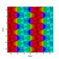
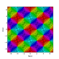
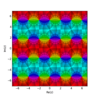
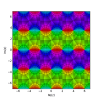
In the complex plane of the argument u, the twelve functions form a repeating lattice of simple poles and zeroes.[1] Depending on the function, one repeating parallelogram, or unit cell, will have sides of length 2K or 4K on the real axis, and 2K' or 4K' on the imaginary axis, where K=K(m) and K'=K(1-m) are known as the quarter periods with K(.) being the elliptic integral of the first kind. The nature of the unit cell can be determined by inspecting the "auxiliary rectangle" (generally a parallelogram), which is a rectangle formed by the origin (0,0) at one corner, and (K,K') as the diagonally opposite corner. As in the diagram, the four corners of the auxiliary rectangle are named s, c, d, and n, going counter-clockwise from the origin. The function pq(u,m) will have a zero at the "p" corner and a pole at the "q" corner. The twelve functions correspond to the twelve ways of arranging these poles and zeroes in the corners of the rectangle.

When the argument u and parameter m are real, with 0<m<1, K and K' will be real and the auxiliary parallelogram will in fact be a rectangle, and the Jacobi elliptic functions will all be real valued on the real line.

Mathematically, Jacobian elliptic functions are doubly periodic meromorphic functions on the complex plane. Since they are doubly periodic, they factor through a torus – in effect, their domain can be taken to be a torus, just as cosine and sine are in effect defined on a circle. Instead of having only one circle, we now have the product of two circles, one real and the other imaginary. The complex plane can be replaced by a complex torus. The circumference of the first circle is 4K and the second 4K′, where K and K′ are the quarter periods. Each function has two zeroes and two poles at opposite positions on the torus. Among the points 0, K, K + iK′, iK′ there is one zero and one pole.

The Jacobian elliptic functions are then the unique doubly periodic, meromorphic functions satisfying the following three properties:

• There is a simple zero at the corner p, and a simple pole at the corner q.
• The step from p to q is equal to half the period of the function pq u; that is, the function pq u is periodic in the direction pq, with the period being twice the distance from p to q. The function pq u is also periodic in the other two directions, with a period such that the distance from p to one of the other corners is a quarter period.
• If the function pq u is expanded in terms of u at one of the corners, the leading term in the expansion has a coefficient of 1. In other words, the leading term of the expansion of pq u at the corner p is u; the leading term of the expansion at the corner q is 1/u, and the leading term of an expansion at the other two corners is 1.

Jacobi elliptic function sn

Jacobi elliptic function cn

Jacobi elliptic function dn

Jacobi elliptic function sc

Plots of four Jacobi Elliptic Functions in the complex plane of ‘’u’’, illustrating their double periodic behavior. Images generated using a version of the domain coloring method.[2] All have values of the k parameter equal to 0.8.

The elliptic functions can be given in a variety of notations, which can make the subject unnecessarily confusing. Elliptic functions are functions of two variables. The first variable might be given in terms of the amplitude φ, or more commonly, in terms of u given below. The second variable might be given in terms of the parameter m, or as the elliptic modulus k, where k² = m, or in terms of the modular angle α, where m =  sin² α. The complements of k and m are defined as m' =1-m and ${\displaystyle k'={\sqrt {m'}}}$. These four terms are used below without comment to simplify various expressions.

The twelve Jacobi elliptic functions are generally written as pq(u,m) where ‘’p’’ and ‘’q’’ are any of the letters ‘’c’’, ‘’s’’, ‘’n’’, and ‘’d’’. Functions of the form pp(u,m) are trivially set to unity for notational completeness. The “major” functions are generally taken to be cn(u,m), sn(u,m) and dn(u,m) from which all other functions can be derived and expressions are often written solely in terms of these three functions, however, various symmetries and generalizations are often most conveniently expressed using the full set. (This notation is due to Gudermann and Glaisher and is not Jacobi's original notation.)

The parameter

The functions are notationally related to each other by the multiplication rule: (arguments suppressed)

${\displaystyle \operatorname {pq} \,\,\,\,\operatorname {p'q'} =\operatorname {pq'} \,\,\,\operatorname {p'q} }$

from which other commonly used relationships can be derived:

${\displaystyle \operatorname {pr} /\operatorname {qr} =\operatorname {pq} }$

${\displaystyle \operatorname {pr} \,\,\operatorname {rq} =\operatorname {pq} }$

${\displaystyle 1/\operatorname {qp} =\operatorname {pq} }$

The multiplication rule follows immediately from the identification of the elliptic functions with the Neville theta functions[3]

${\displaystyle \operatorname {pq} (u,m)={\frac {\theta _{p}(u,m)}{\theta _{q}(u,m)}}}$

Model of amplitude (measured along vertical axis) as a function of independent variables u and k

The above definition, in terms of the unique meromorphic functions satisfying certain properties, is quite abstract. There is a simpler, but completely equivalent definition, giving the elliptic functions as inverses of the incomplete elliptic integral of the first kind. Let

${\displaystyle u=\int _{0}^{\varphi }{\frac {\mathrm {d} \theta }{\sqrt {1-m\sin ^{2}\theta }}}\,.}$

Then the elliptic sine sn u (Latin: sinus amplitudinis) is given by

${\displaystyle \operatorname {sn} u=\sin \varphi \,}$

and the elliptic cosine cn u (Latin: cosinus amplitudinis) is given by

${\displaystyle \operatorname {cn} u=\cos \varphi }$

and the delta amplitude dn u (Latin: delta amplitudinis)

${\displaystyle \operatorname {dn} u={\sqrt {1-m\sin ^{2}\varphi }}\,.}$

Here, the angle ${\displaystyle \varphi }$ is called the amplitude. On occasion, dn u = Δ(u) is called the delta amplitude. In the above, the value m is a free parameter, usually taken to be real, 0 ≤ m ≤ 1, and so the elliptic functions can be thought of as being given by two variables, the amplitude ${\displaystyle \varphi }$ and the parameter m.

The remaining nine elliptic functions are easily built from the above three, and are given in a section below.

Note that when ${\displaystyle \varphi =\pi /2}$, that u then equals the quarter period K.

Plot of the Jacobi ellipse (x²+y²/b²=1, b real) and the twelve Jacobi Elliptic functions pq(u,m) for particular values of angle φ and parameter b. The solid curve is the ellipse, with m=1-1/b² and u=F(φ,m) where F(.,.) is the elliptic integral of the first kind. The dotted curve is the unit circle. Tangent lines from the circle and ellipse at x=cd crossing the x-axis at dc are shown in light grey.

${\displaystyle \cos \varphi ,\sin \varphi }$ are defined on the unit circle, with radius r = 1 and angle ${\displaystyle \varphi =}$ arc length of the unit circle measured from the positive x-axis. Similarly, Jacobi elliptic functions are defined on the unit ellipse, with a = 1. Let

${\displaystyle {\begin{aligned}&x^{2}+{\frac {y^{2}}{b^{2}}}=1,\quad b>1,\\&m=1-{\frac {1}{b^{2}}},\quad 0<m<1,\\&x=r\cos \varphi ,\quad y=r\sin \varphi \end{aligned}}}$

then:

${\displaystyle r(\varphi ,m)={\frac {1}{\sqrt {1-m\sin ^{2}\varphi }}}\,.}$

For each angle ${\displaystyle \varphi }$ the angular component of the arc length, the 'angular arc length' is computed. An advantage of angular arc length is that we can calculate a total arc length for hyperbolas. For the ellipse the angular arc length is:

${\displaystyle u=u(\varphi ,m)=\int _{0}^{\varphi }r(\theta ,m)\,d\theta .}$

Let ${\displaystyle P=(x,y)}$ be the point on the ellipse with angular arc length ${\displaystyle u(\varphi ,m)}$ and let ${\displaystyle P'=(x',y')}$ be the point on the unit circle with the angular arc length ${\displaystyle \varphi }$, (note that origin ${\displaystyle O,P'}$ and ${\displaystyle P}$ are on the same straight line). The familiar relations from the unit circle (${\displaystyle OP'=1}$):

${\displaystyle x'=\cos \varphi ,\quad y'=\sin \varphi }$

imply for the ellipse:

${\displaystyle x'=\operatorname {cn} (u,m),\quad y'=\operatorname {sn} (u,m).}$

So the projections of the intersection point ${\displaystyle P'}$ of the line ${\displaystyle OP}$ with the unit circle on the x- and y-axes are simply ${\displaystyle \operatorname {cn} (u,m)}$ and ${\displaystyle \operatorname {sn} (u,m)}$. These projections may be interpreted as 'definition as trigonometry'. In short:

${\displaystyle \operatorname {cn} (u,m)={\frac {x(u,m)}{r(u,m)}},\quad \operatorname {sn} (u,m)={\frac {y(u,m)}{r(u,m)}},\quad \operatorname {dn} (u,m)={\frac {1}{r(u,m)}}.}$

For the ${\displaystyle x}$ and ${\displaystyle y}$ value of the point ${\displaystyle P}$ with ${\displaystyle u}$ and parameter ${\displaystyle m}$ we get, after inserting the relation:

${\displaystyle r(\varphi ,m)={\frac {1}{\operatorname {dn} (u,m)}}}$

into:${\displaystyle x=r(\varphi ,m)\cos(\varphi ),y=r(\varphi ,m)\sin(\varphi )}$ that:

${\displaystyle x={\frac {\operatorname {cn} (u,m)}{\operatorname {dn} (u,m)}},\quad y={\frac {\operatorname {sn} (u,m)}{\operatorname {dn} (u,m)}}.}$

The latter relations for the x- and y-coordinates of points on the unit ellipse may be considered as generalization of the relations ${\displaystyle x=\cos \varphi ,y=\sin \varphi }$ for the coordinates of points on the unit circle.

The following table summarizes the expressions for all Jacobi elliptic functions pq(u,m) in the variables (x,y,r) and (φ,dn) with ${\displaystyle r={\sqrt {x^{2}+y^{2}}}}$

Jacobi Elliptic Functions pq[u,m] as functions of {x,y,r} and {φ,dn}

		q
		c	s	n	d
p
	c	1	${\displaystyle x/y=\cot(\phi )}$	${\displaystyle x/r=\cos(\phi )}$	${\displaystyle x=\cos(\phi )/dn}$
	s	${\displaystyle y/x=\tan(\phi )}$	1	${\displaystyle y/r=\sin(\phi )}$	${\displaystyle y=\sin(\phi )/dn}$
	n	${\displaystyle r/x=\sec(\phi )}$	${\displaystyle r/y=\csc(\phi )}$	1	${\displaystyle r=1/dn}$
	d	${\displaystyle 1/x=dn\sec(\phi )}$	${\displaystyle 1/y=dn\csc(\phi )}$	${\displaystyle 1/r=dn}$	1

Equivalently, Jacobi's elliptic functions can be defined in terms of his theta functions. If we abbreviate ${\displaystyle \vartheta (0;\tau )}$ as ${\displaystyle \vartheta }$, and ${\displaystyle \vartheta _{01}(0;\tau ),\vartheta _{10}(0;\tau ),\vartheta _{11}(0;\tau )}$ respectively as ${\displaystyle \vartheta _{01},\vartheta _{10},\vartheta _{11}}$ (the theta constants) then the elliptic modulus k is ${\displaystyle k=\left({\vartheta _{10} \over \vartheta }\right)^{2}}$. If we set ${\displaystyle u=\pi \vartheta ^{2}z}$, we have

${\displaystyle {\begin{aligned}\operatorname {sn} (u;k)&=-{\vartheta \vartheta _{11}(z;\tau ) \over \vartheta _{10}\vartheta _{01}(z;\tau )}\\[7pt]\operatorname {cn} (u;k)&={\vartheta _{01}\vartheta _{10}(z;\tau ) \over \vartheta _{10}\vartheta _{01}(z;\tau )}\\[7pt]\operatorname {dn} (u;k)&={\vartheta _{01}\vartheta (z;\tau ) \over \vartheta \vartheta _{01}(z;\tau )}\end{aligned}}}$

Since the Jacobi functions are defined in terms of the elliptic modulus ${\displaystyle k(\tau )}$, we need to invert this and find ${\displaystyle \tau }$ in terms of ${\displaystyle k}$. We start from ${\displaystyle k'={\sqrt {1-k^{2}}}}$, the complementary modulus. As a function of ${\displaystyle \tau }$ it is

${\displaystyle k'(\tau )=\left({\vartheta _{01} \over \vartheta }\right)^{2}.}$

Let us first define

${\displaystyle \ell ={1 \over 2}{1-{\sqrt {k'}} \over 1+{\sqrt {k'}}}={1 \over 2}{\vartheta -\vartheta _{01} \over \vartheta +\vartheta _{01}}.}$

Then define the nome as ${\displaystyle q=\exp(\pi i\tau )}$ and expand ${\displaystyle \ell }$ as a power series in the nome ${\displaystyle q}$, we obtain

${\displaystyle \ell ={q+q^{9}+q^{25}+\cdots \over 1+2q^{4}+2q^{16}+\cdots }.}$

Reversion of series now gives

${\displaystyle q=\ell +2\ell ^{5}+15\ell ^{9}+150\ell ^{13}+1707\ell ^{17}+20910\ell ^{21}+268616\ell ^{25}+\cdots .}$

Since we may reduce to the case where the imaginary part of ${\displaystyle \tau }$ is greater than or equal to ${\displaystyle {\sqrt {3}}/2}$, we can assume the absolute value of ${\displaystyle q}$ is less than or equal to ${\displaystyle \exp(-\pi {\sqrt {3}}/2)\approx 0.0658}$; for values this small the above series converges very rapidly and easily allows us to find the appropriate value for ${\displaystyle q}$.

The Jacobi elliptic functions can be defined very simply using the Neville theta functions:[4]

${\displaystyle pq(u,m)={\frac {\theta _{p}(u,m)}{\theta _{q}(u,m)}}}$

Simplifications of complicated products of the Jacobi elliptic functions are often made easier using these identities.

Plot of the Jacobi hyperbola (x²+y²/b²=1, b imaginary) and the twelve Jacobi Elliptic functions pq(u,m) for particular values of angle φ and parameter b. The solid curve is the hyperbola, with m=1-1/b² and u=F(φ,m) where F(.,.) is the elliptic integral of the first kind. The dotted curve is the unit circle. For the ds-dc triangle,σ= Sin(φ)Cos(φ).

Introducing complex numbers, our ellipse has an associated hyperbola:

${\displaystyle xx^{2}-{\frac {yy^{2}}{b^{2}}}=1}$

from applying Jacobi's imaginary transformation[4] to the elliptic functions in the above equation for x and y.

${\displaystyle xx={\frac {1}{\operatorname {dn} (u,1-m)}},\quad yy={\frac {\operatorname {sn} (u,1-m)}{\operatorname {dn} (u,1-m)}}}$

It follows that we can put ${\displaystyle x=\operatorname {dn} (u,1-m),y=\operatorname {sn} (u,1-m)}$. So our ellipse has a dual ellipse with m replaced by 1-m. This leads to the complex torus mentioned in the Introduction.[6] Generally, m may be a complex number, but when m is real and m<0, the curve is an ellipse with major axis in the x direction. At m=0 the curve is a circle, and for 0<m<1, the curve is an ellipse with major axis in the y direction. At m=1, the curve degenerates into two vertical lines at x=+/- 1. For m>1, the curve is a hyperbola. When m is complex but not real, x or y or both are complex and the curve cannot be described on a real x-y diagram.

Reversing the order of the two letters of the function name results in the reciprocals of the three functions above:

${\displaystyle {\begin{aligned}\operatorname {ns} (u)={\frac {1}{\operatorname {sn} (u)}},\qquad \operatorname {nc} (u)={\frac {1}{\operatorname {cn} (u)}},\qquad \operatorname {nd} (u)={\frac {1}{\operatorname {dn} (u)}}.\end{aligned}}}$

Similarly, the ratios of the three primary functions correspond to the first letter of the numerator followed by the first letter of the denominator:

${\displaystyle {\begin{aligned}\operatorname {sc} (u)={\frac {\operatorname {sn} (u)}{\operatorname {cn} (u)}},\qquad \operatorname {sd} (u)={\frac {\operatorname {sn} (u)}{\operatorname {dn} (u)}},\qquad \operatorname {dc} (u)={\frac {\operatorname {dn} (u)}{\operatorname {cn} (u)}},\qquad \operatorname {ds} (u)={\frac {\operatorname {dn} (u)}{\operatorname {sn} (u)}},\qquad \operatorname {cs} (u)={\frac {\operatorname {cn} (u)}{\operatorname {sn} (u)}},\qquad \operatorname {cd} (u)={\frac {\operatorname {cn} (u)}{\operatorname {dn} (u)}}.\end{aligned}}}$

More compactly, we have

${\displaystyle \operatorname {pq} (u)={\frac {\operatorname {pn} (u)}{\operatorname {qn} (u)}}}$

where p and q are any of the letters s, c, d.

Plots of the phase for the twelve Jacobi Elliptic functions pq(u,m) as a function complex argument u, with poles and zeroes indicated. The plots are over one full cycle in the real and imaginary directions with the colored portion indicating phase according to the color wheel at the lower right (which replaces the trivial dd function). Regions with amplitude below 1/3 are colored black, roughly indicating the location of a zero, while regions with amplitude above 3 are colored white, roughly indicating the position of a pole. All plots use m=2/3 with K=K(m), K'=K(1-m), K(.) being the complete elliptic integral of the first kind. Arrows at the poles point in direction of zero phase. Right and left arrows imply positive and negative real residues respectively. Up and down arrows imply positive and negative imaginary residues respectively.

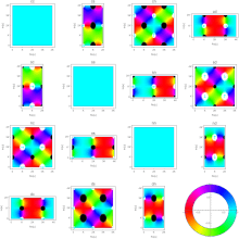
In the complex plane of the argument u, the Jacobi elliptic functions form a repeating pattern of poles (and zeroes). The residues of the poles all have the same amplitude, differing only in sign. Each function pq(u,m) has an inverse function qp(u,m) in which the positions of the poles and zeroes are exchanged. The periods of repetition are generally different in the real and imaginary directions, hence the use of the term "doubly periodic" to describe them.

The double periodicity of the Jacobi elliptic functions may be expressed as:

${\displaystyle \operatorname {pq} (u+2\alpha K(m)+2i\beta K(1-m)\,,\,m)=(-1)^{\gamma }\operatorname {pq} (u,m)}$

where α and β are any pair of integers. K(.) is the complete elliptic integral of the first kind, also known as the quarter period. The power of negative unity (γ) is given in the following table:

${\displaystyle \gamma }$

		q
		c	s	n	d
p
	c	0	β	α+β	α
	s	β	0	α	α+β
	n	α+β	α	0	β
	d	α	α+β	β	0

When the factor (-1)^γ is equal to -1, the equation expresses quasi-periodicity. When it is equal to unity, it expresses full periodicity. It can be seen, for example, that for the entries containing only α when α is even, full periodicity is expressed by the above equation, and the function has full periods of 4K(m) and 2iK(1-m). Likewise, functions with entries containing only β have full periods of 2K(m) and 4iK(1-m), while those with α + β have full periods of 4K(m) and 4iK(1-m).

In the diagram on the right, which plots one repeating unit for each function, indicating phase along with the location of poles and zeroes, a number of regularities can be noted: The inverse of each function is opposite the diagonal, and has the same size unit cell, with poles and zeroes exchanged. The pole and zero arrangement in the auxiliary rectangle formed by (0,0), (K,0), (0,K') and (K,K') are in accordance with the description of the pole and zero placement described in the introduction above. Also, the size of the white ovals indicating poles are a rough measure of the amplitude of the residue for that pole. The residues of the poles closest to the origin in the figure (i.e. in the auxiliary rectangle) are listed in the following table:

Residues of Jacobi Elliptic Functions

		q
		c	s	n	d
p
	c		1	${\displaystyle -{\frac {i}{k}}}$	${\displaystyle -{\frac {1}{k}}}$
	s	${\displaystyle -{\frac {1}{k'}}}$		${\displaystyle {\frac {1}{k}}}$	${\displaystyle -{\frac {i}{k\,k'}}}$
	n	${\displaystyle -{\frac {1}{k'}}}$	1		${\displaystyle -{\frac {i}{k'}}}$
	d	-1	1	${\displaystyle -i}$

When applicable, poles displaced above by 2K or displaced to the right by 2K' have the same value but with signs reversed, while those diagonally opposite have the same value. Note that poles and zeroes on the left and lower edges are considered part of the unit cell, while those on the upper and right edges are not.

Relations between squares of the functions can be derived from two basic relationships (Arguments (u,m) suppressed):

${\displaystyle \operatorname {cn} ^{2}+\operatorname {sn} ^{2}=1}$

${\displaystyle \operatorname {cn} ^{2}+m'\operatorname {sn} ^{2}=\operatorname {dn} ^{2}}$

where m + m' = 1 and m = k². Multiplying by any function of the form nq yields more general equations:

${\displaystyle \operatorname {cq} ^{2}+\operatorname {sq} ^{2}=\operatorname {nq} ^{2}}$

${\displaystyle \operatorname {cq} ^{2}+m'\operatorname {sq} ^{2}=\operatorname {dq} ^{2}}$

With q=d, these correspond trigonometrically to the equations for the unit circle (${\displaystyle x^{2}+y^{2}=r^{2}}$) and the unit ellipse (${\displaystyle x^{2}+m'y^{2}=1}$), with x=cd, y=sd and r=nd. Using the multiplication rule, other relationships may be derived. For example:

${\displaystyle -\operatorname {dn} ^{2}+m'=-m\operatorname {cn} ^{2}=m\operatorname {sn} ^{2}-m}$

${\displaystyle -m'\operatorname {nd} ^{2}+m'=-mm'\operatorname {sd} ^{2}=m\operatorname {cd} ^{2}-m}$

${\displaystyle m'\operatorname {sc} ^{2}+m'=m'\operatorname {nc} ^{2}=\operatorname {dc} ^{2}-m}$

${\displaystyle \operatorname {cs} ^{2}+m'=\operatorname {ds} ^{2}=\operatorname {ns} ^{2}-m}$

The functions satisfy the two square relations

${\displaystyle \operatorname {cn} ^{2}(u,k)+\operatorname {sn} ^{2}(u,k)=1,\,}$

${\displaystyle \operatorname {dn} ^{2}(u,k)+k^{2}\operatorname {sn} ^{2}(u,k)=1.\,}$

From this we see that (cn, sn, dn) parametrizes an elliptic curve which is the intersection of the two quadrics defined by the above two equations. We now may define a group law for points on this curve by the addition formulas for the Jacobi functions[1]

${\displaystyle {\begin{aligned}\operatorname {cn} (x+y)&={\operatorname {cn} (x)\operatorname {cn} (y)-\operatorname {sn} (x)\operatorname {sn} (y)\operatorname {dn} (x)\operatorname {dn} (y) \over {1-k^{2}\operatorname {sn} ^{2}(x)\operatorname {sn} ^{2}(y)}},\\[8pt]\operatorname {sn} (x+y)&={\operatorname {sn} (x)\operatorname {cn} (y)\operatorname {dn} (y)+\operatorname {sn} (y)\operatorname {cn} (x)\operatorname {dn} (x) \over {1-k^{2}\operatorname {sn} ^{2}(x)\operatorname {sn} ^{2}(y)}},\\[8pt]\operatorname {dn} (x+y)&={\operatorname {dn} (x)\operatorname {dn} (y)-k^{2}\operatorname {sn} (x)\operatorname {sn} (y)\operatorname {cn} (x)\operatorname {cn} (y) \over {1-k^{2}\operatorname {sn} ^{2}(x)\operatorname {sn} ^{2}(y)}}.\end{aligned}}}$

Double angle formulae can be easily derived from the above equations by setting x=y.[1] Half angle formulae[4][1] are all of the form:

${\displaystyle \operatorname {pq} ({\tfrac {1}{2}}u,m)^{2}=f_{p}/f_{q}}$

where:

${\displaystyle f_{c}=\operatorname {cn} (u,m)+\operatorname {dn} (u,m)}$

${\displaystyle f_{s}=1-\operatorname {cn} (u,m)}$

${\displaystyle f_{n}=1+\operatorname {dn} (u,m)}$

${\displaystyle f_{d}=(1+\operatorname {dn} (u,m))-m(1-\operatorname {cn} (u,m))}$

Let the nome be ${\displaystyle q=\exp(-\pi K'/K)}$ and let the argument be ${\displaystyle v=\pi u/(2K)}$. Then the functions have expansions as Lambert series

${\displaystyle \operatorname {sn} (u)={\frac {2\pi }{K{\sqrt {m}}}}\sum _{n=0}^{\infty }{\frac {q^{n+1/2}}{1-q^{2n+1}}}\sin((2n+1)v),}$

${\displaystyle \operatorname {cn} (u)={\frac {2\pi }{K{\sqrt {m}}}}\sum _{n=0}^{\infty }{\frac {q^{n+1/2}}{1+q^{2n+1}}}\cos((2n+1)v),}$

${\displaystyle \operatorname {dn} (u)={\frac {\pi }{2K}}+{\frac {2\pi }{K}}\sum _{n=1}^{\infty }{\frac {q^{n}}{1+q^{2n}}}\cos(2nv).}$

The derivatives of the three basic Jacobi elliptic functions are:

${\displaystyle {\frac {\mathrm {d} }{\mathrm {d} z}}\operatorname {sn} (z)=\operatorname {cn} (z)\operatorname {dn} (z),}$

${\displaystyle {\frac {\mathrm {d} }{\mathrm {d} z}}\operatorname {cn} (z)=-\operatorname {sn} (z)\operatorname {dn} (z),}$

${\displaystyle {\frac {\mathrm {d} }{\mathrm {d} z}}\operatorname {dn} (z)=-k^{2}\operatorname {sn} (z)\operatorname {cn} (z).}$

These can be used to derive the derivatives of all other functions as shown in the table below (arguments (u,m) suppressed):

Derivatives ${\displaystyle {\frac {d}{du}}\operatorname {pq} (u,m)}$

		q
		c	s	n	d
p
	c	0	-ds ns	-dn sn	-m' nd sd
	s	dc nc	0	cn dn	cd nd
	n	dc sc	-cs ds	0	m cd sd
	d	m' nc sc	-cs ns	-m cn sn	0

With the addition theorems above and for a given k with 0 < k < 1 the major functions are therefore solutions to the following nonlinear ordinary differential equations:

• ${\displaystyle \operatorname {sn} (x)}$ solves the differential equations

${\displaystyle {\frac {\mathrm {d} ^{2}y}{\mathrm {d} x^{2}}}+(1+k^{2})y-2k^{2}y^{3}=0}$

and

${\displaystyle \left({\frac {\mathrm {d} y}{\mathrm {d} x}}\right)^{2}=(1-y^{2})(1-k^{2}y^{2})}$

• ${\displaystyle \operatorname {cn} (x)}$ solves the differential equations

${\displaystyle {\frac {\mathrm {d} ^{2}y}{\mathrm {d} x^{2}}}+(1-2k^{2})y+2k^{2}y^{3}=0}$

and

${\displaystyle \left({\frac {\mathrm {d} y}{\mathrm {d} x}}\right)^{2}=(1-y^{2})(1-k^{2}+k^{2}y^{2})}$

• ${\displaystyle \operatorname {dn} (x)}$ solves the differential equations

${\displaystyle {\frac {\mathrm {d} ^{2}y}{\mathrm {d} x^{2}}}-(2-k^{2})y+2y^{3}=0}$

and

${\displaystyle \left({\frac {\mathrm {d} y}{\mathrm {d} x}}\right)^{2}=(y^{2}-1)(1-k^{2}-y^{2})}$

The Jacobi elliptic functions can be expanded in terms of the hyperbolic functions. When ${\displaystyle m}$ is close to unity, such that ${\displaystyle m'^{2}}$ and higher powers of ${\displaystyle m'}$ can be neglected, we have:

• sn(u):

${\displaystyle \operatorname {sn} (u,m)\approx \tanh(u)+{\frac {1}{4}}m'(\sinh(u)\cosh(u)-u)\operatorname {sech} ^{2}(u).}$

• cn(u):

${\displaystyle \operatorname {cn} (u,m)\approx \operatorname {sech} (u)-{\frac {1}{4}}m'(\sinh(u)\cosh(u)-u)\tanh u\operatorname {sech} (u).}$

• dn(u):

${\displaystyle \operatorname {dn} (u,m)\approx \operatorname {sech} (u)+{\frac {1}{4}}m'(\sinh(u)\cosh(u)+u)\tanh(u)\operatorname {sech} (u).}$

• am(u):

${\displaystyle \operatorname {am} (u,m)\approx \operatorname {gd} (u)+{\frac {1}{4}}m'(\sinh(u)\cosh(u)-u)\operatorname {sech} (u).}$

The inverses of the Jacobi elliptic functions can be defined similarly to the inverse trigonometric functions; if ${\displaystyle x=\operatorname {sn} (\xi ,k)}$, ${\displaystyle \xi =\mathrm {arcsn} (x,k)}$. They can be represented as elliptic integrals,[7][8][9] and power series representations have been found.[10][1]

• ${\displaystyle \mathrm {arcsn} \,(x,k)=\int _{0}^{x}{\frac {\mathrm {d} t}{\sqrt {(1-t^{2})(1-k^{2}t^{2})}}}}$
• ${\displaystyle \mathrm {arccn} \,(x,k)=\int _{x}^{1}{\frac {\mathrm {d} t}{\sqrt {(1-t^{2})(1-k^{2}+k^{2}t^{2})}}}}$
• ${\displaystyle \mathrm {arcdn} \,(x,k)=\int _{x}^{1}{\frac {\mathrm {d} t}{\sqrt {(1-t^{2})(t^{2}+k^{2}-1)}}}}$

The Peirce quincuncial projection is a map projection based on Jacobian elliptic functions.

• Elliptic curve
• Schwarz–Christoffel mapping
• Carlson symmetric form
• Jacobi theta function
• Ramanujan theta function
• Dixon elliptic functions
• Abel elliptic functions
• Weierstrass's elliptic functions

• Abramowitz, Milton; Stegun, Irene Ann, eds. (1983) [June 1964]. "Chapter 16". Handbook of Mathematical Functions with Formulas, Graphs, and Mathematical Tables. Applied Mathematics Series. 55 (Ninth reprint with additional corrections of tenth original printing with corrections (December 1972); first ed.). Washington D.C.; New York: United States Department of Commerce, National Bureau of Standards; Dover Publications. p. 569. ISBN 978-0-486-61272-0. LCCN 64-60036. MR 0167642. LCCN 65-12253.
• N. I. Akhiezer, Elements of the Theory of Elliptic Functions, (1970) Moscow, translated into English as AMS Translations of Mathematical Monographs Volume 79 (1990) AMS, Rhode Island ISBN 0-8218-4532-2
• A. C. Dixon The elementary properties of the elliptic functions, with examples (Macmillan, 1894)
• Alfred George Greenhill The applications of elliptic functions (London, New York, Macmillan, 1892)
• H. Hancock Lectures on the theory of elliptic functions (New York, J. Wiley & sons, 1910)
• Jacobi, C. G. J. (1829), Fundamenta nova theoriae functionum ellipticarum (in Latin), Königsberg, ISBN 978-1-108-05200-9, Reprinted by Cambridge University Press 2012
• Reinhardt, William P.; Walker, Peter L. (2010), "Jacobian Elliptic Functions", in Olver, Frank W. J.; Lozier, Daniel M.; Boisvert, Ronald F.; Clark, Charles W. (eds.), NIST Handbook of Mathematical Functions, Cambridge University Press, ISBN 978-0-521-19225-5, MR 2723248
• (in French) P. Appell and E. Lacour Principes de la théorie des fonctions elliptiques et applications (Paris, Gauthier Villars, 1897)
• (in French) G. H. Halphen Traité des fonctions elliptiques et de leurs applications (vol. 1) (Paris, Gauthier-Villars, 1886–1891)
• (in French) G. H. Halphen Traité des fonctions elliptiques et de leurs applications (vol. 2) (Paris, Gauthier-Villars, 1886–1891)
• (in French) G. H. Halphen Traité des fonctions elliptiques et de leurs applications (vol. 3) (Paris, Gauthier-Villars, 1886–1891)
• (in French) J. Tannery and J. Molk Eléments de la théorie des fonctions elliptiques. Tome I, Introduction. Calcul différentiel. Ire partie (Paris : Gauthier-Villars et fils, 1893)
• (in French) J. Tannery and J. Molk Eléments de la théorie des fonctions elliptiques. Tome II, Calcul différentiel. IIe partie (Paris : Gauthier-Villars et fils, 1893)
• (in French) J. Tannery and J. Molk Eléments de la théorie des fonctions elliptiques. Tome III, Calcul intégral. Ire partie, Théorèmes généraux. Inversion (Paris : Gauthier-Villars et fils, 1893)
• (in French) J. Tannery and J. Molk Eléments de la théorie des fonctions elliptiques. Tome IV, Calcul intégral. IIe partie, Applications (Paris : Gauthier-Villars et fils, 1893)
• (in French) C. Briot and J. C. Bouquet Théorie des fonctions elliptiques ( Paris : Gauthier-Villars, 1875)

• Hazewinkel, Michiel, ed. (2001) [1994], "Jacobi elliptic functions", Encyclopedia of Mathematics, Springer Science+Business Media B.V. / Kluwer Academic Publishers, ISBN 978-1-55608-010-4
• Weisstein, Eric W. "Jacobi Elliptic Functions". MathWorld.
• Elliptic Functions and Elliptic Integrals on YouTube, lecture by William A. Schwalm (4 hours)