Heapsort
In computer science, heapsort is a comparison-based sorting algorithm. Heapsort can be thought of as an improved selection sort: like selection sort, heapsort divides its input into a sorted and an unsorted region, and it iteratively shrinks the unsorted region by extracting the largest element from it and inserting it into the sorted region. Unlike selection sort, heapsort does not waste time with a linear-time scan of the unsorted region; rather, heap sort maintains the unsorted region in a heap data structure to more quickly find the largest element in each step.[1]
 A run of heapsort sorting an array of randomly permuted values. In the first stage of the algorithm the array elements are reordered to satisfy the heap property. Before the actual sorting takes place, the heap tree structure is shown briefly for illustration. | |
| Class | Sorting algorithm |
|---|---|
| Data structure | Array |
| Worst-case performance | |
| Best-case performance | (distinct keys) or (equal keys) |
| Average performance | |
| Worst-case space complexity | total auxiliary |


Although somewhat slower in practice on most machines than a well-implemented quicksort, it has the advantage of a more favorable worst-case O(n log n) runtime. Heapsort is an in-place algorithm, but it is not a stable sort.
Heapsort was invented by J. W. J. Williams in 1964.[2] This was also the birth of the heap, presented already by Williams as a useful data structure in its own right.[3] In the same year, R. W. Floyd published an improved version that could sort an array in-place, continuing his earlier research into the treesort algorithm.[3]
Overview
The heapsort algorithm can be divided into two parts.
In the first step, a heap is built out of the data (see Binary heap § Building a heap). The heap is often placed in an array with the layout of a complete binary tree. The complete binary tree maps the binary tree structure into the array indices; each array index represents a node; the index of the node's parent, left child branch, or right child branch are simple expressions. For a zero-based array, the root node is stored at index 0; if i is the index of the current node, then
  iParent(i)     = floor((i-1) / 2) where floor functions map a real number to the smallest leading integer.
  iLeftChild(i)  = 2*i + 1
  iRightChild(i) = 2*i + 2
In the second step, a sorted array is created by repeatedly removing the largest element from the heap (the root of the heap), and inserting it into the array. The heap is updated after each removal to maintain the heap property. Once all objects have been removed from the heap, the result is a sorted array.
Heapsort can be performed in place. The array can be split into two parts, the sorted array and the heap. The storage of heaps as arrays is diagrammed here. The heap's invariant is preserved after each extraction, so the only cost is that of extraction.
Algorithm
The Heapsort algorithm involves preparing the list by first turning it into a max heap. The algorithm then repeatedly swaps the first value of the list with the last value, decreasing the range of values considered in the heap operation by one, and sifting the new first value into its position in the heap. This repeats until the range of considered values is one value in length.
The steps are:
- Call the buildMaxHeap() function on the list. Also referred to as heapify(), this builds a heap from a list in O(n) operations.
- Swap the first element of the list with the final element. Decrease the considered range of the list by one.
- Call the siftDown() function on the list to sift the new first element to its appropriate index in the heap.
- Go to step (2) unless the considered range of the list is one element.
The buildMaxHeap() operation is run once, and is O(n) in performance. The siftDown() function is O(log n), and is called n times. Therefore, the performance of this algorithm is O(n + n log n) = O(n log n).
Pseudocode
The following is a simple way to implement the algorithm in pseudocode. Arrays are zero-based and swap is used to exchange two elements of the array. Movement 'down' means from the root towards the leaves, or from lower indices to higher. Note that during the sort, the largest element is at the root of the heap at a[0], while at the end of the sort, the largest element is in a[end].
procedure heapsort(a, count) is
    input: an unordered array a of length count

    (Build the heap in array a so that largest value is at the root)
    heapify(a, count)

    (The following loop maintains the invariants that a[0:end] is a heap and every element
     beyond end is greater than everything before it (so a[end:count] is in sorted order))
    end ← count - 1
    while end > 0 do
        (a[0] is the root and largest value. The swap moves it in front of the sorted elements.)
        swap(a[end], a[0])
        (the heap size is reduced by one)
        end ← end - 1
        (the swap ruined the heap property, so restore it)
        siftDown(a, 0, end)
The sorting routine uses two subroutines, heapify and siftDown. The former is the common in-place heap construction routine, while the latter is a common subroutine for implementing heapify.
(Put elements of 'a' in heap order, in-place)
procedure heapify(a, count) is
    (start is assigned the index in 'a' of the last parent node)
    (the last element in a 0-based array is at index count-1; find the parent of that element)
    start ← iParent(count-1)

    while start ≥ 0 do
        (sift down the node at index 'start' to the proper place such that all nodes below
         the start index are in heap order)
        siftDown(a, start, count - 1)
        (go to the next parent node)
        start ← start - 1
    (after sifting down the root all nodes/elements are in heap order)

(Repair the heap whose root element is at index 'start', assuming the heaps rooted at its children are valid)
procedure siftDown(a, start, end) is
    root ← start

    while iLeftChild(root) ≤ end do    (While the root has at least one child)
        child ← iLeftChild(root)   (Left child of root)
        swap ← root                (Keeps track of child to swap with)

        if a[swap] < a[child] then
            swap ← child
        (If there is a right child and that child is greater)
        if child+1 ≤ end and a[swap] < a[child+1] then
            swap ← child + 1
        if swap = root then
            (The root holds the largest element. Since we assume the heaps rooted at the
             children are valid, this means that we are done.)
            return
        else
            swap(a[root], a[swap])
            root ← swap            (repeat to continue sifting down the child now)
The heapify procedure can be thought of as building a heap from the bottom up by successively sifting downward to establish the heap property. An alternative version (shown below) that builds the heap top-down and sifts upward may be simpler to understand. This siftUp version can be visualized as starting with an empty heap and successively inserting elements, whereas the siftDown version given above treats the entire input array as a full but "broken" heap and "repairs" it starting from the last non-trivial sub-heap (that is, the last parent node).
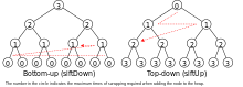
Also, the siftDown version of heapify has O(n) time complexity, while the siftUp version given below has O(n log n) time complexity due to its equivalence with inserting each element, one at a time, into an empty heap.[4]
This may seem counter-intuitive since, at a glance, it is apparent that the former only makes half as many calls to its logarithmic-time sifting function as the latter; i.e., they seem to differ only by a constant factor, which never affects asymptotic analysis.
To grasp the intuition behind this difference in complexity, note that the number of swaps that may occur during any one siftUp call increases with the depth of the node on which the call is made. The crux is that there are many (exponentially many) more "deep" nodes than there are "shallow" nodes in a heap, so that siftUp may have its full logarithmic running-time on the approximately linear number of calls made on the nodes at or near the "bottom" of the heap. On the other hand, the number of swaps that may occur during any one siftDown call decreases as the depth of the node on which the call is made increases. Thus, when the siftDown heapify begins and is calling siftDown on the bottom and most numerous node-layers, each sifting call will incur, at most, a number of swaps equal to the "height" (from the bottom of the heap) of the node on which the sifting call is made. In other words, about half the calls to siftDown will have at most only one swap, then about a quarter of the calls will have at most two swaps, etc.
The heapsort algorithm itself has O(n log n) time complexity using either version of heapify.
 procedure heapify(a,count) is
     (end is assigned the index of the first (left) child of the root)
     end := 1

     while end < count
         (sift up the node at index end to the proper place such that all nodes above
          the end index are in heap order)
         siftUp(a, 0, end)
         end := end + 1
     (after sifting up the last node all nodes are in heap order)

 procedure siftUp(a, start, end) is
     input:  start represents the limit of how far up the heap to sift.
                   end is the node to sift up.
     child := end
     while child > start
         parent := iParent(child)
         if a[parent] < a[child] then (out of max-heap order)
             swap(a[parent], a[child])
             child := parent (repeat to continue sifting up the parent now)
         else
             return
Variations
Floyd's heap construction
The most important variation to the basic algorithm, which is included in all practical implementations, is a heap-construction algorithm by Floyd which runs in O(n) time and uses siftdown rather than siftup, avoiding the need to implement siftup at all.
Rather than starting with a trivial heap and repeatedly adding leaves, Floyd's algorithm starts with the leaves, observing that they are trivial but valid heaps by themselves, and then adds parents. Starting with element n/2 and working backwards, each internal node is made the root of a valid heap by sifting down. The last step is sifting down the first element, after which the entire array obeys the heap property.
The worst-case number of comparisons during the Floyd's heap-construction phase of Heapsort is known to be equal to 2n − 2s2(n) − e2(n), where s2(n) is the number of 1 bits in the binary representation of n and e2(n) is number of trailing 0 bits.[5]
The standard implementation of Floyd's heap-construction algorithm causes a large number of cache misses once the size of the data exceeds that of the CPU cache. Much better performance on large data sets can be obtained by merging in depth-first order, combining subheaps as soon as possible, rather than combining all subheaps on one level before proceeding to the one above.[6][7]
Bottom-up heapsort
Bottom-up heapsort is a variant which reduces the number of comparisons required by a significant factor. While ordinary heapsort requires 2n log2n + O(n) comparisons worst-case and on average,[8] the bottom-up variant requires n log2n + O(1) comparisons on average,[8] and 1.5n log2n + O(n) in the worst case.[9]
If comparisons are cheap (e.g. integer keys) then the difference is unimportant,[10] as top-down heapsort compares values that have already been loaded from memory. If, however, comparisons require a function call or other complex logic, then bottom-up heapsort is advantageous.
This is accomplished by improving the siftDown procedure. The change improves the linear-time heap-building phase somewhat,[11] but is more significant in the second phase. Like ordinary heapsort, each iteration of the second phase extracts the top of the heap, a[0], and fills the gap it leaves with a[end], then sifts this latter element down the heap. But this element comes from the lowest level of the heap, meaning it is one of the smallest elements in the heap, so the sift-down will likely take many steps to move it back down. In ordinary heapsort, each step of the sift-down requires two comparisons, to find the minimum of three elements: the new node and its two children.
Bottom-up heapsort instead finds the path of largest children to the leaf level of the tree (as if it were inserting −∞) using only one comparison per level. Put another way, it finds a leaf which has the property that it and all of its ancestors are greater than or equal to their siblings. (In the absence of equal keys, this leaf is unique.) Then, from this leaf, it searches upward (using one comparison per level) for the correct position in that path to insert a[end]. This is the same location as ordinary heapsort finds, and requires the same number of exchanges to perform the insert, but fewer comparisons are required to find that location.[9]
Because it goes all the way to the bottom and then comes back up, it is called heapsort with bounce by some authors.[12]
function leafSearch(a, i, end) is
    j ← i
    while iRightChild(j) ≤ end do
        (Determine which of j's two children is the greater)
        if a[iRightChild(j)] > a[iLeftChild(j)] then
            j ← iRightChild(j)
        else
            j ← iLeftChild(j)
    (At the last level, there might be only one child)
    if iLeftChild(j) ≤ end then
        j ← iLeftChild(j)
    return j
The return value of the leafSearch is used in the modified siftDown routine:[9]
procedure siftDown(a, i, end) is
    j ← leafSearch(a, i, end)
    while a[i] > a[j] do
        j ← iParent(j)
    x ← a[j]
    a[j] ← a[i]
    while j > i do
        swap x, a[iParent(j)]
        j ← iParent(j)
Bottom-up heapsort was announced as beating quicksort (with median-of-three pivot selection) on arrays of size ≥16000.[8]
A 2008 re-evaluation of this algorithm showed it to be no faster than ordinary heapsort for integer keys, presumably because modern branch prediction nullifies the cost of the predictable comparisons which bottom-up heapsort manages to avoid.[10]
A further refinement does a binary search in the path to the selected leaf, and sorts in a worst case of (n+1)(log2(n+1) + log2 log2(n+1) + 1.82) + O(log2n) comparisons, approaching the information-theoretic lower bound of n log2n − 1.4427n comparisons.[13]
A variant which uses two extra bits per internal node (n−1 bits total for an n-element heap) to cache information about which child is greater (two bits are required to store three cases: left, right, and unknown)[11] uses less than n log2n + 1.1n compares.[14]
Other variations
- Ternary heapsort[15] uses a ternary heap instead of a binary heap; that is, each element in the heap has three children. It is more complicated to program, but does a constant number of times fewer swap and comparison operations. This is because each sift-down step in a ternary heap requires three comparisons and one swap, whereas in a binary heap two comparisons and one swap are required. Two levels in a ternary heap cover 32 = 9 elements, doing more work with the same number of comparisons as three levels in the binary heap, which only cover 23 = 8. This is primarily of academic interest, as the additional complexity is not worth the minor savings, and bottom-up heapsort beats both.
- The smoothsort algorithm[16] is a variation of heapsort developed by Edsger Dijkstra in 1981. Like heapsort, smoothsort's upper bound is O(n log n). The advantage of smoothsort is that it comes closer to O(n) time if the input is already sorted to some degree, whereas heapsort averages O(n log n) regardless of the initial sorted state. Due to its complexity, smoothsort is rarely used.
- Levcopoulos and Petersson[17] describe a variation of heapsort based on a heap of Cartesian trees. First, a Cartesian tree is built from the input in O(n) time, and its root is placed in a 1-element binary heap. Then we repeatedly extract the minimum from the binary heap, output the tree's root element, and add its left and right children (if any) which are themselves Cartesian trees, to the binary heap.[18] As they show, if the input is already nearly sorted, the Cartesian trees will be very unbalanced, with few nodes having left and right children, resulting in the binary heap remaining small, and allowing the algorithm to sort more quickly than O(n log n) for inputs that are already nearly sorted.
- Several variants such as weak heapsort require n log2n+O(1) comparisons in the worst case, close to the theoretical minimum, using one extra bit of state per node. While this extra bit makes the algorithms not truly in-place, if space for it can be found inside the element, these algorithms are simple and efficient,[6]:40 but still slower than binary heaps if key comparisons are cheap enough (e.g. integer keys) that a constant factor does not matter.[19]
- Katajainen's "ultimate heapsort" requires no extra storage, performs n log2n+O(1) comparisons, and a similar number of element moves.[20] It is, however, even more complex and not justified unless comparisons are very expensive.
Comparison with other sorts
Heapsort primarily competes with quicksort, another very efficient general purpose nearly-in-place comparison-based sort algorithm.
Quicksort is typically somewhat faster due to some factors, but the worst-case running time for quicksort is O(n2), which is unacceptable for large data sets and can be deliberately triggered given enough knowledge of the implementation, creating a security risk. See quicksort for a detailed discussion of this problem and possible solutions.
Thus, because of the O(n log n) upper bound on heapsort's running time and constant upper bound on its auxiliary storage, embedded systems with real-time constraints or systems concerned with security often use heapsort, such as the Linux kernel.[21]
Heapsort also competes with merge sort, which has the same time bounds. Merge sort requires Ω(n) auxiliary space, but heapsort requires only a constant amount. Heapsort typically runs faster in practice on machines with small or slow data caches, and does not require as much external memory. On the other hand, merge sort has several advantages over heapsort:
- Merge sort on arrays has considerably better data cache performance, often outperforming heapsort on modern desktop computers because merge sort frequently accesses contiguous memory locations (good locality of reference); heapsort references are spread throughout the heap.
- Heapsort is not a stable sort; merge sort is stable.
- Merge sort parallelizes well and can achieve close to linear speedup with a trivial implementation; heapsort is not an obvious candidate for a parallel algorithm.
- Merge sort can be adapted to operate on singly linked lists with O(1) extra space. Heapsort can be adapted to operate on doubly linked lists with only O(1) extra space overhead.
- Merge sort is used in external sorting; heapsort is not. Locality of reference is the issue.
Introsort is an alternative to heapsort that combines quicksort and heapsort to retain advantages of both: worst case speed of heapsort and average speed of quicksort.
Example
Let { 6, 5, 3, 1, 8, 7, 2, 4 } be the list that we want to sort from the smallest to the largest. (NOTE, for 'Building the Heap' step: Larger nodes don't stay below smaller node parents. They are swapped with parents, and then recursively checked if another swap is needed, to keep larger numbers above smaller numbers on the heap binary tree.)
| Heap | newly added element | swap elements |
|---|---|---|
| null | 6 | |
| 6 | 5 | |
| 6, 5 | 3 | |
| 6, 5, 3 | 1 | |
| 6, 5, 3, 1 | 8 | |
| 6, 5, 3, 1, 8 | 5, 8 | |
| 6, 8, 3, 1, 5 | 6, 8 | |
| 8, 6, 3, 1, 5 | 7 | |
| 8, 6, 3, 1, 5, 7 | 3, 7 | |
| 8, 6, 7, 1, 5, 3 | 2 | |
| 8, 6, 7, 1, 5, 3, 2 | 4 | |
| 8, 6, 7, 1, 5, 3, 2, 4 | 1, 4 | |
| 8, 6, 7, 4, 5, 3, 2, 1 |
| Heap | swap elements | delete element | sorted array | details |
|---|---|---|---|---|
| 8, 6, 7, 4, 5, 3, 2, 1 | 8, 1 | swap 8 and 1 in order to delete 8 from heap | ||
| 1, 6, 7, 4, 5, 3, 2, 8 | 8 | delete 8 from heap and add to sorted array | ||
| 1, 6, 7, 4, 5, 3, 2 | 1, 7 | 8 | swap 1 and 7 as they are not in order in the heap | |
| 7, 6, 1, 4, 5, 3, 2 | 1, 3 | 8 | swap 1 and 3 as they are not in order in the heap | |
| 7, 6, 3, 4, 5, 1, 2 | 7, 2 | 8 | swap 7 and 2 in order to delete 7 from heap | |
| 2, 6, 3, 4, 5, 1, 7 | 7 | 8 | delete 7 from heap and add to sorted array | |
| 2, 6, 3, 4, 5, 1 | 2, 6 | 7, 8 | swap 2 and 6 as they are not in order in the heap | |
| 6, 2, 3, 4, 5, 1 | 2, 5 | 7, 8 | swap 2 and 5 as they are not in order in the heap | |
| 6, 5, 3, 4, 2, 1 | 6, 1 | 7, 8 | swap 6 and 1 in order to delete 6 from heap | |
| 1, 5, 3, 4, 2, 6 | 6 | 7, 8 | delete 6 from heap and add to sorted array | |
| 1, 5, 3, 4, 2 | 1, 5 | 6, 7, 8 | swap 1 and 5 as they are not in order in the heap | |
| 5, 1, 3, 4, 2 | 1, 4 | 6, 7, 8 | swap 1 and 4 as they are not in order in the heap | |
| 5, 4, 3, 1, 2 | 5, 2 | 6, 7, 8 | swap 5 and 2 in order to delete 5 from heap | |
| 2, 4, 3, 1, 5 | 5 | 6, 7, 8 | delete 5 from heap and add to sorted array | |
| 2, 4, 3, 1 | 2, 4 | 5, 6, 7, 8 | swap 2 and 4 as they are not in order in the heap | |
| 4, 2, 3, 1 | 4, 1 | 5, 6, 7, 8 | swap 4 and 1 in order to delete 4 from heap | |
| 1, 2, 3, 4 | 4 | 5, 6, 7, 8 | delete 4 from heap and add to sorted array | |
| 1, 2, 3 | 1, 3 | 4, 5, 6, 7, 8 | swap 1 and 3 as they are not in order in the heap | |
| 3, 2, 1 | 3, 1 | 4, 5, 6, 7, 8 | swap 3 and 1 in order to delete 3 from heap | |
| 1, 2, 3 | 3 | 4, 5, 6, 7, 8 | delete 3 from heap and add to sorted array | |
| 1, 2 | 1, 2 | 3, 4, 5, 6, 7, 8 | swap 1 and 2 as they are not in order in the heap | |
| 2, 1 | 2, 1 | 3, 4, 5, 6, 7, 8 | swap 2 and 1 in order to delete 2 from heap | |
| 1, 2 | 2 | 3, 4, 5, 6, 7, 8 | delete 2 from heap and add to sorted array | |
| 1 | 1 | 2, 3, 4, 5, 6, 7, 8 | delete 1 from heap and add to sorted array | |
| 1, 2, 3, 4, 5, 6, 7, 8 | completed |
Notes
- Skiena, Steven (2008). "Searching and Sorting". The Algorithm Design Manual. Springer. p. 109. doi:10.1007/978-1-84800-070-4_4. ISBN 978-1-84800-069-8.
[H]eapsort is nothing but an implementation of selection sort using the right data structure.
- Williams 1964
- Brass, Peter (2008). Advanced Data Structures. Cambridge University Press. p. 209. ISBN 978-0-521-88037-4.
- "Priority Queues". Retrieved 24 May 2011.
- Suchenek, Marek A. (2012), "Elementary Yet Precise Worst-Case Analysis of Floyd's Heap-Construction Program", Fundamenta Informaticae, 120 (1): 75–92, doi:10.3233/FI-2012-751
- Bojesen, Jesper; Katajainen, Jyrki; Spork, Maz (2000). "Performance Engineering Case Study: Heap Construction" (PostScript). ACM Journal of Experimental Algorithmics. 5 (15): 15–es. CiteSeerX 10.1.1.35.3248. doi:10.1145/351827.384257. Alternate PDF source.
- Chen, Jingsen; Edelkamp, Stefan; Elmasry, Amr; Katajainen, Jyrki (27–31 August 2012). In-place Heap Construction with Optimized Comparisons, Moves, and Cache Misses (PDF). 37th international conference on Mathematical Foundations of Computer Science. Bratislava, Slovakia. pp. 259–270. doi:10.1007/978-3-642-32589-2_25. ISBN 978-3-642-32588-5. See particularly Fig. 3.
- Wegener, Ingo (13 September 1993). "BOTTOM-UP HEAPSORT, a new variant of HEAPSORT beating, on an average, QUICKSORT (if n is not very small)" (PDF). Theoretical Computer Science. 118 (1): 81–98. doi:10.1016/0304-3975(93)90364-y. Although this is a reprint of work first published in 1990 (at the Mathematical Foundations of Computer Science conference), the technique was published by Carlsson in 1987.[13]
- Fleischer, Rudolf (February 1994). "A tight lower bound for the worst case of Bottom-Up-Heapsort" (PDF). Algorithmica. 11 (2): 104–115. doi:10.1007/bf01182770. hdl:11858/00-001M-0000-0014-7B02-C. Also available as Fleischer, Rudolf (April 1991). A tight lower bound for the worst case of Bottom-Up-Heapsort (PDF) (Technical report). MPI-INF. MPI-I-91-104.
- Mehlhorn, Kurt; Sanders, Peter (2008). "Priority Queues" (PDF). Algorithms and Data Structures: The Basic Toolbox. Springer. p. 142. ISBN 978-3-540-77977-3.
- McDiarmid, C.J.H.; Reed, B.A. (September 1989). "Building heaps fast" (PDF). Journal of Algorithms. 10 (3): 352–365. doi:10.1016/0196-6774(89)90033-3.
- Moret, Bernard; Shapiro, Henry D. (1991). "8.6 Heapsort". Algorithms from P to NP Volume 1: Design and Efficiency. Benjamin/Cummings. p. 528. ISBN 0-8053-8008-6.
For lack of a better name we call this enhanced program 'heapsort with bounce.'
- Carlsson, Scante (March 1987). "A variant of heapsort with almost optimal number of comparisons" (PDF). Information Processing Letters. 24 (4): 247–250. doi:10.1016/0020-0190(87)90142-6.
- Wegener, Ingo (March 1992). "The worst case complexity of McDiarmid and Reed's variant of BOTTOM-UP HEAPSORT is less than n log n + 1.1n". Information and Computation. 97 (1): 86–96. doi:10.1016/0890-5401(92)90005-Z.
- "Data Structures Using Pascal", 1991, page 405, gives a ternary heapsort as a student exercise. "Write a sorting routine similar to the heapsort except that it uses a ternary heap."
- Dijkstra, Edsger W. Smoothsort – an alternative to sorting in situ (EWD-796a) (PDF). E.W. Dijkstra Archive. Center for American History, University of Texas at Austin. (transcription)
- Levcopoulos, Christos; Petersson, Ola (1989), "Heapsort—Adapted for Presorted Files", WADS '89: Proceedings of the Workshop on Algorithms and Data Structures, Lecture Notes in Computer Science, 382, London, UK: Springer-Verlag, pp. 499–509, doi:10.1007/3-540-51542-9_41, ISBN 978-3-540-51542-5 Heapsort—Adapted for presorted files (Q56049336).
- Schwartz, Keith (27 December 2010). "CartesianTreeSort.hh". Archive of Interesting Code. Retrieved 5 March 2019.
- Katajainen, Jyrki (23 September 2013). Seeking for the best priority queue: Lessons learnt. Algorithm Engineering (Seminar 13391). Dagstuhl. pp. 19–20, 24.
- Katajainen, Jyrki (2–3 February 1998). The Ultimate Heapsort. Computing: the 4th Australasian Theory Symposium. Australian Computer Science Communications. 20 (3). Perth. pp. 87–96.
- https://github.com/torvalds/linux/blob/master/lib/sort.c Linux kernel source
References
- Williams, J. W. J. (1964), "Algorithm 232 - Heapsort", Communications of the ACM, 7 (6): 347–348, doi:10.1145/512274.512284
- Floyd, Robert W. (1964), "Algorithm 245 - Treesort 3", Communications of the ACM, 7 (12): 701, doi:10.1145/355588.365103
- Carlsson, Svante (1987), "Average-case results on heapsort", BIT, 27 (1): 2–17, doi:10.1007/bf01937350
- Knuth, Donald (1997), "§5.2.3, Sorting by Selection", Sorting and Searching, The Art of Computer Programming, 3 (third ed.), Addison-Wesley, pp. 144–155, ISBN 978-0-201-89685-5
- Thomas H. Cormen, Charles E. Leiserson, Ronald L. Rivest, and Clifford Stein. Introduction to Algorithms, Second Edition. MIT Press and McGraw-Hill, 2001. ISBN 0-262-03293-7. Chapters 6 and 7 Respectively: Heapsort and Priority Queues
- A PDF of Dijkstra's original paper on Smoothsort
- Heaps and Heapsort Tutorial by David Carlson, St. Vincent College
External links
| The Wikibook Algorithm implementation has a page on the topic of: Heapsort |
- Animated Sorting Algorithms: Heap Sort at the Wayback Machine (archived 6 March 2015) – graphical demonstration
- Courseware on Heapsort from Univ. Oldenburg - With text, animations and interactive exercises
- NIST's Dictionary of Algorithms and Data Structures: Heapsort
- Heapsort implemented in 12 languages
- Sorting revisited by Paul Hsieh
- A PowerPoint presentation demonstrating how Heap sort works that is for educators.
- Open Data Structures - Section 11.1.3 - Heap-Sort, Pat Morin