Fairness (machine learning)
In machine learning, a given algorithm is said to be fair, or to have fairness if its results are independent of some variables we consider to be sensitive and not related with it (f.e.: gender, ethnicity, sexual orientation, etc.).
Context
Research about fairness in machine learning is a relatively recent topic. Most of the articles about it have been written in the last three years[1]. Some of the most important facts in this topic are the following:
- In 2018, IBM introduces AI Fairness 360, a Python library with several algorithms to reduce bias in a program, increasing its fairness.[2]
- Facebook made public, in 2018, their use of a tool, Fairness Flow, to detect bias in their AI. However, said tool code is not accessible, and it is not known if it really corrects this bias.[3]
- In 2019, Google publishes a set of tools in Github to study the effects of fairness in the long run.[4]
The algorithms used for assuring fairness are still being improved. However, the main progress in this area is that some big corporations are realizing the importance of the reduction of algorithm bias will have on society.
Fairness criteria in classification problems[5]
In classification problems, an algorithm learns a function to predict a discrete characteristic , the target variable, from known characteristics . We model as a discrete random variable which encodes some characteristics contained or implicitly encoded in that we consider as sensitive characteristics (gender, ethnicity, sexual orientation, etc.). We finally denote by the prediction of the classifier. Now let us define three main criteria to evaluate if a given classifier is fair, that is, if its predictions are not influenced by some of these sensitive variables.


Independence
We say the random variables satisfy independence if the sensitive characteristics are statistically independent to the prediction , and we write .


We can also express this notion with the following formula:

This means that the probability of being classified by the algorithm in each of the groups is equal for two individuals with different sensitive characteristics.
Yet another equivalent expression for independence can be given using the concept of mutual information between random variables, defined as

In this formula, of the random variable. Then satisfy independence if .


A possible relaxation of the indepence definition include introducing a positive slack and is given by the formula:


Finally, another possible relaxation is to require .

Separation
We say the random variables satisfy separation if the sensitive characteristics are statistically independent to the prediction given the target value , and we write .


We can also express this notion with the following formula:

This means that the probability of being classified by the algorithm in each of the groups is equal for two individuals with different sensitive characteristics given that they actually belong in the same group (have the same target variable).
Another equivalent expression, in the case of a binary target rate, is that the true positive rate and the false positive rate are equal (and therefore the false negative rate and the true negative rate are equal) for every value of the sensitive characteristics:


Finally, a possible relaxation of the given definitions is the difference between rates to be a positive number lower than a given slack , instead of equals to zero.
Sufficiency
We say the random variables satisfy sufficiency if the sensitive characteristics are statistically independent to the target value given the prediction , and we write .

We can also express this notion with the following formula:

This means that the probability of actually being in each of the groups is equal for two individuals with different sensitive characteristics given that they were predicted to belong to the same group.
Relationships between definitions
Finally, we sum up some of the main results that relate the three definitions given above:
- If and are not statistically independent, then sufficiency and independence cannot both hold.
- Assuming is binary, if and are not statistically independent, and and are not statistically independent either, then independence and separation cannot both hold.
- If as a joint distribution has positive probability for all its possible values and and are not statistically independent, then separation and sufficiency cannot both hold.
Metrics[6]
Most statistical measures of fairness rely on different metrics, so we will start by defining them. When working with a binary classifier, both the predicted and the actual classes can take two values: positive and negative. Now let us start explaining the different possible relations between predicted and actual outcome:
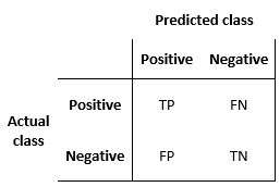
- True positive (TP): The case where both the predicted and the actual outcome are in a positive class.
- True negative (TN): The case where both the predicted and the actual outcome are in the negative class.
- False positive (FP): A case predicted to be in a positive class when the actual outcome is in the negative one.
- False negative (FN): A case predicted to be in the negative class when the actual outcome is in the positive one.
These relations can be easily represented with a confusion matrix, a table that describes the accuracy of a classification model. In this matrix, columns and rows represent instances of the predicted and the actual cases, respectively.
By using this relations, we can define multiple metrics which can be later used to measure the fairness of an algorithm:
- Positive predicted value (PPV): the fraction of positive cases which were correctly predicted out of all the positive predictions. It is usually referred to as precision, and represents the probability of a positive prediction to be right. It is given by the following formula:

- False discovery rate (FDR): the fraction of positive predictions which were actually negative out of all the positive predictions. It represents the probability of a positive prediction to be wrong, and it is given by the following formula:

- Negative predicted value (NPV): the fraction of negative cases which were correctly predicted out of all the negative predictions. It represents the probability of a negative prediction to be right, and it is given by the following formula:

- False omission rate (FOR): the fraction of negative predictions which were actually positive out of all the negative predictions. It represents the probability of a negative prediction to be wrong, and it is given by the following formula:

- True positive rate (TPR): the fraction of positive cases which were correctly predicted out of all the positive cases. It is usually referred to as sensitivity or recall, and it represents the probability of the positive subjects to be classified correctly as such. It is given by the formula:

- False negative rate (FNR): the fraction of positive cases which were incorrectly predicted to be negative out of all the positive cases. It represents the probability of the positive subjects to be classified incorrectly as negative ones, and it is given by the formula:

- True negative rate (TNR): the fraction of negative cases which were correctly predicted out of all the negative cases. It represents the probability of the negative subjects to be classified correctly as such, and it is given by the formula:

- False positive rate (FPR): the fraction of negative cases which were incorrectly predicted to be positive out of all the negative cases. It represents the probability of the negative subjects to be classified incorrectly as positive ones, and it is given by the formula:

Other fairness criteria

The following criteria can be understood as measures of the three definitions given in the first section, or relaxation of them. In the table[5] to the right, we can see the relationships between them.
To define these measures specifically, we will divide them into three big groups as done in Verma et al.[6]: definitions based on a predicted outcome, on predicted and actual outcomes, and definitions based on predicted probabilities and the actual outcome.
We will be working with a binary classifier and the following notation: refers to the score given by the classifier, which is the probability of a certain subject to be in the positive or the negative class. represents the final classification predicted by the algorithm, and its value is usually derived from , for example will be positive when is above a certain threshold. represents the actual outcome, that is, the real classification of the individual and, finally, denotes the sensitive attributes of the subjects.

Definitions based on predicted outcome
The definitions in this section focus on a predicted outcome for various distributions of subjects. They are the simplest and most intuitive notions of fairness.
- Group fairness, also referred to as statistical parity, demographic parity, acceptance rate and benchmarking. A classifier satisfies this definition if the subjects in the protected and unprotected groups have equal probability of being assigned to the positive predicted class. This is, if the following formula is satisfied:

- Conditional statistical parity. Basically consists in the definition above, but restricted only to a subset of the attributes. With mathematical notation this would be:

Definitions based on predicted and actual outcomes
This definitions not only consider de predicted outcome but also compare it to the actual outcome .
- Predictive parity, also referred to as outcome test. A classifier satisfies this definition if the subjects in the protected and unprotected groups have equal PPV. This is, if the following formula is satisfied:

- Mathematically, if a classifier has equal PPV for both groups, it will also have equal FDR, satisfying the formula:

- False positive error rate balance, also referred to as predictive equality. A classifier satisfies this definition if the subjects in the protected and unprotected groups have aqual FPR. This is, if the following formula is satisfied:

- Mathematically, if a classifier has equal FPR for both groups, it will also have equal TNR, satisfying the formula:

- False negative error rate balance, also referred to as equal opportunity. A classifier satisfies this definition if the subjects in the protected and unprotected groups have equal FNR. This is, if the following formula is satisfied:

- Mathematically, if a classifier has equal FNR for both groups, ti will also have equal TPR, satisfying the formula:

- Equalized odds, also referred to as conditional procedure accuracy equality and disparate mistreatment. A classifier satisfies this definition if the subjects in the protected and unprotected groups have equal TPR and equal FPR, satisfying the formula:

- Conditional use accuracy equality. A classifier satisfies this definition if the subjects in the protected and unprotected groups have equal PPV and equal NPV, satisfying the formula:

- Overall accuracy equality. A classifier satisfies this definition if the subject in the protected and unprotected groups have equal prediction accuracy, that is, the probability of a subject from one class to be assigned to it. This is, if it satisfies the following formula:

- Treatment equality. A classifier satisfies this definition if the subjects in the protected and unprotected groups have an equal ratio of FN and FP, satisfying the formula:

Definitions based on predicted probabilities and actual outcome
These definitions are based in the actual outcome and the predicted probability score .
- Test-fairness, also known as calibration or matching conditional frequencies. A classifier satisfies this definition if individuals with the same predicted probability score have the same probability to be classified in the positive class when they belong to either the protected or the unprotected group:

- Well-calibration is an extension of the previous definition. It states that when individuals inside or outside the protected group have the same predicted probability score they must have the same probability of being classified in the positive class, and this probability must be equal to :

- Balance for positive class. A classifier satisfies this definition if the subjects constituting the positive class from both protected and unprotected groups have equal average predicted probability score . This means that the expected value of probability score for the protected and unprotected groups with positive actual outcome is the same, satisfying the formula:

- Balance for negative class. A classifier satisfies this definition if the subjects constituting the negative class from both protected and unprotected groups have equal average predicted probability score . This means that the expected value of probability score for the protected and unprotected groups with negative actual outcome is the same, satisfying the formula:

Algorithms
Fairness can be applied to machine learning algorithms in three different ways: preprocessing the data used in the algorithm, optimization during the training, or post-processing the answers of the algorithm.
Preprocessing
Usually, the classifier is not the only problem, the dataset is also biased. The discrimination of a dataset with respect to the group can be defined as follows:


That is, an approximation to the difference between the probabilities of belonging in the positive class given that the subject has a protected characteristic different from and equal to .

Algorithms correcting bias at preprocessing remove information concerning variables in the dataset which can result in unfair decisions of the AI, while trying to alter just the bare minimum of this data. This is not as easy as just removing the sensitive variable, because other attributes can be related to the protected one.
A way to do this is by mapping each individual in the initial dataset into an intermediate representation in which it is impossible to identify whether it belongs to a particular protected group while maintaining as much information as possible. Then, the new representation of the data is adjusted to get the maximum accuracy in the algorithm.
This way, individuals are mapped into a new multivariable representation where the probability of any member of a protected group to be mapped to a certain value in the new representation is the same as the probability of an individual which doesn't belong to the protected group. Then, this representation is used to obtain the prediction for the individual, instead of the initial data. As the intermediate representation is constructed giving the same probability to individuals inside or outside the protected group, this attribute is hidden to the classificator.
An example is explained in Zemel et al.[7] where a multinomial random variable is used as an intermediate representation. In the process, the system is encouraged to preserve all the information except those that can lead to biased decisions and to obtain a prediction as accurate as possible.
On the one hand, this procedure has the advantage that the preprocessed data can be used for any machine learning task. Furthermore, the classifier does not need to be modified, as the correction is applied to the dataset before processing. On the other hand, the other methods obtain better results in accuracy and fairness.[8]
Reweighing[9]
Reweighing is an example of a preprocessing algorithm. The idea is to assign a weight to each dataset point such that the weighted discrimination is 0 with respect to the designated group.
If the dataset was unbiased the sensitive variable and the target variable would be statistically independent and the probability of the joint distribution would be the product of the probabilities as follows:

In reality, however, the dataset is not unbiased and the variables are not statistically independent so the observed probability is:

To compensate for the bias, lower weights to favored objects and higher weights to unfavored objects will be assigned. For each we get:


When we have for each a weight associated we compute the weighted discrimination with respect to group as follows:


It can be shown that after reweighting this weighted discrimination is 0.
Optimization at training time
Another approach is correcting the bias at training time. This can be done by adding constraints to the optimization objective of the algorithm.[10] These constraints force the algorithm to improve fairness, by keeping the same rates of certain measures for the protected group and the rest of individuals. For example, we can add to the objective of the algorithm the condition that the false positive rate is the same for individuals in the protected group and the ones outside the protected group.
The main measures used in this approach are false positive rate, false negative rate, and overall misclassification rate. It is possible to add just one or several of these constraints to the objective of the algorithm. Note that the equality of false negative rates implies the equality of true positive rates so this implies the equality of opportunity. After adding the restrictions to the problem it may turn intractable, so a relaxation on them may be needed.
This technique obtains good results in improving fairness while keeping high accuracy and lets the programmer choose the fairness measures to improve. However, each machine learning task may need a different method to be applied and the code in the classifier needs to be modified, which is not always possible.[8]
Adversarial debiasing[11][12]
We train two classifiers at the same time through some gradient-based method (f.e.: gradient descent). The first one, the predictor tries to accomplish the task of predicting , the target variable, given , the input, by modifying its weights to minimize some loss function . The second one, the adversary tries to accomplish the task of predicting , the sensitive variable, given by modifying its weights to minimize some loss function .


An important point here is that, in order to propagate correctly, above must refer to the raw output of the classifier, not the discrete prediction; for example, with an artificial neural network and a classification problem, could refer to the output of the softmax layer.
Then we update to minimize at each training step according to the gradient and we modify according to the expression:


where is a tuneable hyperparameter that can vary at each time step.


The intuitive idea is that we want the predictor to try to minimize (therefore the term ) while, at the same time, maximize (therefore the term ), so that the adversary fails at predicting the sensitive variable from .


The term prevents the predictor from moving in a direction that helps the adversary decrease its loss function.

It can be shown that training a predictor classification model with this algorithm improves demographic parity with respect to training it without the adversary.
Postprocessing
The final method tries to correct the results of a classifier to achieve fairness. In this method, we have a classifier that returns a score for each individual and we need to do a binary prediction for them. High scores are likely to get a positive answer, while low scores are likely to get a negative answer, but we need to adjust the threshold to determine when to answer yes or no depending on our needs. Note that variations in the threshold affect the trade-off between true positive rate and true negative rate.
If the score function is fair in the sense that it is independent of the protected attribute, then any choice of the threshold will also be fair, but this type of classifiers tend to be biased, so we may need to set a different threshold for each protected group to achieve fairness. A way to do this is plotting the true positive rate against the false negative rate at various threshold settings (this is called ROC curve) and check which threshold satisfies that the rates are equal for the protected group and the rest of the individuals.[13]
The advantages of postprocessing include that the technique can be applied after any classifiers, without modifying it, and has a good performance in fairness measures. The cons are the need to access to the protected attribute in test time and the lack of choice in the balance between accuracy and fairness.[8]
Reject Option based Classification[14]
Given a classifier let be the probability computed by the classifiers as the probability that the instance belongs to the positive class +. When is close to 1 or to 0, the instance is specified with high degree of certainty to belong to class + or - respectively. However, when is closer to 0.5 the classification is more unclear.

We say is a "rejected instance" if with a certain such that .


The algorithm of "ROC" consists on classifying the non-rejected instances following the rule above and the rejected instances as follows: if the instance is an example of a deprived group () then label it as positive, otherwise, label it as negative.

We can optimize different measures of discrimination (link) as functions of to find the optimal for each problem and avoid becoming discriminatory against the privileged group.
See also
References
- Moritz Hardt, Berkeley. Retrieved 18 December 2019
- IBM AI Fairness 360. Retrieved 18 December 2019
- Fairness Flow el detector de sesgos de Facebook. Retrieved 28 December 2019
- ML-Fairness gym. Retrieved 18 December 2019
- Solon Barocas; Moritz Hardt; Arvind Narayanan, Fairness and Machine Learning. Retrieved 15 December 2019.
- Sahil Verma; Julia Rubin, Fairness Definitions Explained. Retrieved 15 December 2019
- Richard Zemel; Yu (Ledell) Wu; Kevin Swersky; Toniann Pitassi; Cyntia Dwork, Learning Fair Representations. Retrieved 1 December 2019
- Ziyuan Zhong, Tutorial on Fairness in Machine Learning. Retrieved 1 December 2019
- Faisal Kamiran; Toon Calders, Data preprocessing techniques for classification without discrimination. Retrieved 17 December 2019
- Muhammad Bilal Zafar; Isabel Valera; Manuel Gómez Rodríguez; Krishna P. Gummadi, Fairness Beyond Disparate Treatment & Disparate Impact: Learning Classification without Disparate Mistreatment. Retrieved 1 December 2019
- Brian Hu Zhang; Blake Lemoine; Margaret Mitchell, Mitigating Unwanted Biases with Adversarial Learning. Retrieved 17 December 2019
- Joyce Xu, Algorithmic Solutions to Algorithmic Bias: A Technical Guide. Retrieved 17 December 2019
- Moritz Hardt; Eric Price; Nathan Srebro, Equality of Opportunity in Supervised Learning. Retrieved 1 December 2019
- Faisal Kamiran; Asim Karim; Xiangliang Zhang, Decision Theory for Discrimination-aware Classification. Retrieved 17 December 2019