Bloom filter
A Bloom filter is a space-efficient probabilistic data structure, conceived by Burton Howard Bloom in 1970, that is used to test whether an element is a member of a set. False positive matches are possible, but false negatives are not – in other words, a query returns either "possibly in set" or "definitely not in set." Elements can be added to the set, but not removed (though this can be addressed with the counting Bloom filter variant); the more items added, the larger the probability of false positives.
| Part of a series on |
| Probabilistic data structures |
|---|
| Random trees |
| Related |
Bloom proposed the technique for applications where the amount of source data would require an impractically large amount of memory if "conventional" error-free hashing techniques were applied. He gave the example of a hyphenation algorithm for a dictionary of 500,000 words, out of which 90% follow simple hyphenation rules, but the remaining 10% require expensive disk accesses to retrieve specific hyphenation patterns. With sufficient core memory, an error-free hash could be used to eliminate all unnecessary disk accesses; on the other hand, with limited core memory, Bloom's technique uses a smaller hash area but still eliminates most unnecessary accesses. For example, a hash area only 15% of the size needed by an ideal error-free hash still eliminates 85% of the disk accesses.[1]
More generally, fewer than 10 bits per element are required for a 1% false positive probability, independent of the size or number of elements in the set.[2]
Algorithm description
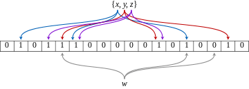
An empty Bloom filter is a bit array of m bits, all set to 0. There must also be k different hash functions defined, each of which maps or hashes some set element to one of the m array positions, generating a uniform random distribution. Typically, k is a small constant which depends on the desired false error rate ε, while m is proportional to k and the number of elements to be added.
To add an element, feed it to each of the k hash functions to get k array positions. Set the bits at all these positions to 1.
To query for an element (test whether it is in the set), feed it to each of the k hash functions to get k array positions. If any of the bits at these positions is 0, the element is definitely not in the set; if it were, then all the bits would have been set to 1 when it was inserted. If all are 1, then either the element is in the set, or the bits have by chance been set to 1 during the insertion of other elements, resulting in a false positive. In a simple Bloom filter, there is no way to distinguish between the two cases, but more advanced techniques can address this problem.
The requirement of designing k different independent hash functions can be prohibitive for large k. For a good hash function with a wide output, there should be little if any correlation between different bit-fields of such a hash, so this type of hash can be used to generate multiple "different" hash functions by slicing its output into multiple bit fields. Alternatively, one can pass k different initial values (such as 0, 1, ..., k − 1) to a hash function that takes an initial value; or add (or append) these values to the key. For larger m and/or k, independence among the hash functions can be relaxed with negligible increase in false positive rate.[3] (Specifically, Dillinger & Manolios (2004b) show the effectiveness of deriving the k indices using enhanced double hashing or triple hashing, variants of double hashing that are effectively simple random number generators seeded with the two or three hash values.)
Removing an element from this simple Bloom filter is impossible because there is no way to tell which of the k bits it maps to should be cleared. Although setting any one of those k bits to zero suffices to remove the element, it would also remove any other elements that happen to map onto that bit. Since the simple algorithm provides no way to determine whether any other elements have been added that affect the bits for the element to be removed, clearing any of the bits would introduce the possibility of false negatives.
One-time removal of an element from a Bloom filter can be simulated by having a second Bloom filter that contains items that have been removed. However, false positives in the second filter become false negatives in the composite filter, which may be undesirable. In this approach re-adding a previously removed item is not possible, as one would have to remove it from the "removed" filter.
It is often the case that all the keys are available but are expensive to enumerate (for example, requiring many disk reads). When the false positive rate gets too high, the filter can be regenerated; this should be a relatively rare event.
Space and time advantages

While risking false positives, Bloom filters have a substantial space advantage over other data structures for representing sets, such as self-balancing binary search trees, tries, hash tables, or simple arrays or linked lists of the entries. Most of these require storing at least the data items themselves, which can require anywhere from a small number of bits, for small integers, to an arbitrary number of bits, such as for strings (tries are an exception since they can share storage between elements with equal prefixes). However, Bloom filters do not store the data items at all, and a separate solution must be provided for the actual storage. Linked structures incur an additional linear space overhead for pointers. A Bloom filter with a 1% error and an optimal value of k, in contrast, requires only about 9.6 bits per element, regardless of the size of the elements. This advantage comes partly from its compactness, inherited from arrays, and partly from its probabilistic nature. The 1% false-positive rate can be reduced by a factor of ten by adding only about 4.8 bits per element.
However, if the number of potential values is small and many of them can be in the set, the Bloom filter is easily surpassed by the deterministic bit array, which requires only one bit for each potential element. Hash tables gain a space and time advantage if they begin ignoring collisions and store only whether each bucket contains an entry; in this case, they have effectively become Bloom filters with k = 1.[4]
Bloom filters also have the unusual property that the time needed either to add items or to check whether an item is in the set is a fixed constant, O(k), completely independent of the number of items already in the set. No other constant-space set data structure has this property, but the average access time of sparse hash tables can make them faster in practice than some Bloom filters. In a hardware implementation, however, the Bloom filter shines because its k lookups are independent and can be parallelized.
To understand its space efficiency, it is instructive to compare the general Bloom filter with its special case when k = 1. If k = 1, then in order to keep the false positive rate sufficiently low, a small fraction of bits should be set, which means the array must be very large and contain long runs of zeros. The information content of the array relative to its size is low. The generalized Bloom filter (k greater than 1) allows many more bits to be set while still maintaining a low false positive rate; if the parameters (k and m) are chosen well, about half of the bits will be set,[5] and these will be apparently random, minimizing redundancy and maximizing information content.
Probability of false positives


Assume that a hash function selects each array position with equal probability. If m is the number of bits in the array, the probability that a certain bit is not set to 1 by a certain hash function during the insertion of an element is

If k is the number of hash functions and each has no significant correlation between each other, then the probability that the bit is not set to 1 by any of the hash functions is

We can use the well-known identity for e−1

to conclude that, for large m,

If we have inserted n elements, the probability that a certain bit is still 0 is

the probability that it is 1 is therefore

Now test membership of an element that is not in the set. Each of the k array positions computed by the hash functions is 1 with a probability as above. The probability of all of them being 1, which would cause the algorithm to erroneously claim that the element is in the set, is often given as

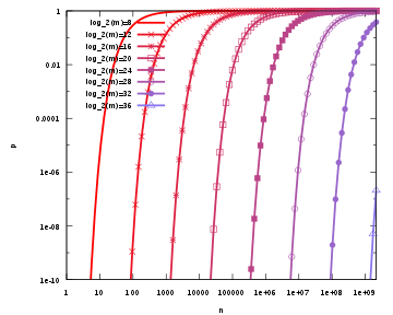
This is not strictly correct as it assumes independence for the probabilities of each bit being set. However, assuming it is a close approximation we have that the probability of false positives decreases as m (the number of bits in the array) increases, and increases as n (the number of inserted elements) increases.
An alternative analysis arriving at the same approximation without the assumption of independence is given by Mitzenmacher and Upfal.[6] After all n items have been added to the Bloom filter, let q be the fraction of the m bits that are set to 0. (That is, the number of bits still set to 0 is qm.) Then, when testing membership of an element not in the set, for the array position given by any of the k hash functions, the probability that the bit is found set to 1 is . So the probability that all k hash functions find their bit set to 1 is . Further, the expected value of q is the probability that a given array position is left untouched by each of the k hash functions for each of the n items, which is (as above)


- .

It is possible to prove, without the independence assumption, that q is very strongly concentrated around its expected value. In particular, from the Azuma–Hoeffding inequality, they prove that[7]

Because of this, we can say that the exact probability of false positives is

as before.
Optimal number of hash functions
The number of hash functions, k, must be a positive integer. Putting this constraint aside, for a given m and n, the value of k that minimizes the false positive probability is

The required number of bits, m, given n (the number of inserted elements) and a desired false positive probability ε (and assuming the optimal value of k is used) can be computed by substituting the optimal value of k in the probability expression above:

which can be simplified to:

This results in:

So the optimal number of bits per element is

with the corresponding number of hash functions k (ignoring integrality):

This means that for a given false positive probability ε, the length of a Bloom filter m is proportionate to the number of elements being filtered n and the required number of hash functions only depends on the target false positive probability ε.[8]
The formula is approximate for three reasons. First, and of least concern, it approximates as , which is a good asymptotic approximation (i.e., which holds as m →∞). Second, of more concern, it assumes that during the membership test the event that one tested bit is set to 1 is independent of the event that any other tested bit is set to 1. Third, of most concern, it assumes that is fortuitously integral.


Goel and Gupta,[9] however, give a rigorous upper bound that makes no approximations and requires no assumptions. They show that the false positive probability for a finite Bloom filter with m bits (), n elements, and k hash functions is at most


This bound can be interpreted as saying that the approximate formula can be applied at a penalty of at most half an extra element and at most one fewer bit.

Approximating the number of items in a Bloom filter
Swamidass & Baldi (2007) showed that the number of items in a Bloom filter can be approximated with the following formula,

where is an estimate of the number of items in the filter, m is the length (size) of the filter, k is the number of hash functions, and X is the number of bits set to one.

The union and intersection of sets
Bloom filters are a way of compactly representing a set of items. It is common to try to compute the size of the intersection or union between two sets. Bloom filters can be used to approximate the size of the intersection and union of two sets. Swamidass & Baldi (2007) showed that for two Bloom filters of length m, their counts, respectively can be estimated as

and

The size of their union can be estimated as

where is the number of bits set to one in either of the two Bloom filters. Finally, the intersection can be estimated as


using the three formulas together.
Interesting properties
- Unlike a standard hash table using open addressing for collision resolution, a Bloom filter of a fixed size can represent a set with an arbitrarily large number of elements; adding an element never fails due to the data structure "filling up." However, the false positive rate increases steadily as elements are added until all bits in the filter are set to 1, at which point all queries yield a positive result. With open addressing hashing, false positives are never produced, but performance steadily deteriorates until it approaches linear search.
- Union and intersection of Bloom filters with the same size and set of hash functions can be implemented with bitwise OR and AND operations, respectively. The union operation on Bloom filters is lossless in the sense that the resulting Bloom filter is the same as the Bloom filter created from scratch using the union of the two sets. The intersect operation satisfies a weaker property: the false positive probability in the resulting Bloom filter is at most the false-positive probability in one of the constituent Bloom filters, but may be larger than the false positive probability in the Bloom filter created from scratch using the intersection of the two sets.
- Some kinds of superimposed code can be seen as a Bloom filter implemented with physical edge-notched cards. An example is Zatocoding, invented by Calvin Mooers in 1947, in which the set of categories associated with a piece of information is represented by notches on a card, with a random pattern of four notches for each category.
Examples
- Fruit flies use a modified version of Bloom filters to detect novelty of odors, with additional features including similarity of novel odor to that of previously experienced examples, and time elapsed since previous experience of the same odor.[10]
- The servers of Akamai Technologies, a content delivery provider, use Bloom filters to prevent "one-hit-wonders" from being stored in its disk caches. One-hit-wonders are web objects requested by users just once, something that Akamai found applied to nearly three-quarters of their caching infrastructure. Using a Bloom filter to detect the second request for a web object and caching that object only on its second request prevents one-hit wonders from entering the disk cache, significantly reducing disk workload and increasing disk cache hit rates.[11]
- Google Bigtable, Apache HBase and Apache Cassandra and PostgreSQL[12] use Bloom filters to reduce the disk lookups for non-existent rows or columns. Avoiding costly disk lookups considerably increases the performance of a database query operation.[13]
- The Google Chrome web browser used to use a Bloom filter to identify malicious URLs. Any URL was first checked against a local Bloom filter, and only if the Bloom filter returned a positive result was a full check of the URL performed (and the user warned, if that too returned a positive result).[14][15]
- Microsoft Bing (search engine) uses multi-level hierarchical Bloom filters for its search index, BitFunnel. Bloom filters provided lower cost than the previous Bing index, which was based on inverted files.[16].
- The Squid Web Proxy Cache uses Bloom filters for cache digests.[17]
- Bitcoin uses Bloom filters to speed up wallet synchronization.[18]
- The Venti archival storage system uses Bloom filters to detect previously stored data.[19]
- The SPIN model checker uses Bloom filters to track the reachable state space for large verification problems.[20]
- The Cascading analytics framework uses Bloom filters to speed up asymmetric joins, where one of the joined data sets is significantly larger than the other (often called Bloom join in the database literature).[21]
- The Exim mail transfer agent (MTA) uses Bloom filters in its rate-limit feature.[22]
- Medium uses Bloom filters to avoid recommending articles a user has previously read.[23]
- Ethereum uses Bloom filters for quickly finding logs on the Ethereum blockchain.
Alternatives
Classic Bloom filters use bits of space per inserted key, where is the false positive rate of the Bloom filter. However, the space that is strictly necessary for any data structure playing the same role as a Bloom filter is only per key.[24] Hence Bloom filters use 44% more space than an equivalent optimal data structure. Instead, Pagh et al. provide an optimal-space data structure. Moreover, their data structure has constant locality of reference independent of the false positive rate, unlike Bloom filters, where a lower false positive rate leads to a greater number of memory accesses per query, . Also, it allows elements to be deleted without a space penalty, unlike Bloom filters. The same improved properties of optimal space usage, constant locality of reference, and the ability to delete elements are also provided by the cuckoo filter of Fan et al. (2014), an open source implementation of which is available.


Stern & Dill (1996) describe a probabilistic structure based on hash tables, hash compaction, which Dillinger & Manolios (2004b) identify as significantly more accurate than a Bloom filter when each is configured optimally. Dillinger and Manolios, however, point out that the reasonable accuracy of any given Bloom filter over a wide range of numbers of additions makes it attractive for probabilistic enumeration of state spaces of unknown size. Hash compaction is, therefore, attractive when the number of additions can be predicted accurately; however, despite being very fast in software, hash compaction is poorly suited for hardware because of worst-case linear access time.
Putze, Sanders & Singler (2007) have studied some variants of Bloom filters that are either faster or use less space than classic Bloom filters. The basic idea of the fast variant is to locate the k hash values associated with each key into one or two blocks having the same size as processor's memory cache blocks (usually 64 bytes). This will presumably improve performance by reducing the number of potential memory cache misses. The proposed variants have however the drawback of using about 32% more space than classic Bloom filters.
The space efficient variant relies on using a single hash function that generates for each key a value in the range where is the requested false positive rate. The sequence of values is then sorted and compressed using Golomb coding (or some other compression technique) to occupy a space close to bits. To query the Bloom filter for a given key, it will suffice to check if its corresponding value is stored in the Bloom filter. Decompressing the whole Bloom filter for each query would make this variant totally unusable. To overcome this problem the sequence of values is divided into small blocks of equal size that are compressed separately. At query time only half a block will need to be decompressed on average. Because of decompression overhead, this variant may be slower than classic Bloom filters but this may be compensated by the fact that a single hash function need to be computed.


Another alternative to classic Bloom filter is the cuckoo filter, based on space-efficient variants of cuckoo hashing. In this case, a hash table is constructed, holding neither keys nor values, but short fingerprints (small hashes) of the keys. If looking up the key finds a matching fingerprint, then key is probably in the set. One useful property of cuckoo filters is that they are updatable; entries may be dynamically added (with a small probability of failure due to the hash table being full) and removed.
Graf & Lemire (2019) describes an approach called an xor filter, where they store fingerprints in a particular type of perfect hash table, producing a filter which is more memory efficient ( bits per key) and faster than Bloom or cuckoo filters. (The time saving comes from the fact that a lookup requires exactly three memory accesses, which can all execute in parallel.) However, filter creation is more complex than Bloom and cuckoo filters, and it is not possible to modify the set after creation.

Extensions and applications
There are over 60 variants of Bloom filters, many surveys of the field, and a continuing churn of applications (see e.g., Luo, et al [25]). Some of the variants differ sufficiently from the original proposal to be breaches from or forks of the original data structure and its philosophy.[26] A treatment which unifies Bloom filters with other work on random projections, compressive sensing, and locality sensitive hashing remains to be done (though see Dasgupta, et al[27] for one attempt inspired by neuroscience).
Cache filtering
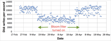
Content delivery networks deploy web caches around the world to cache and serve web content to users with greater performance and reliability. A key application of Bloom filters is their use in efficiently determining which web objects to store in these web caches. Nearly three-quarters of the URLs accessed from a typical web cache are "one-hit-wonders" that are accessed by users only once and never again. It is clearly wasteful of disk resources to store one-hit-wonders in a web cache, since they will never be accessed again. To prevent caching one-hit-wonders, a Bloom filter is used to keep track of all URLs that are accessed by users. A web object is cached only when it has been accessed at least once before, i.e., the object is cached on its second request. The use of a Bloom filter in this fashion significantly reduces the disk write workload, since one-hit-wonders are never written to the disk cache. Further, filtering out the one-hit-wonders also saves cache space on disk, increasing the cache hit rates.[11]
Avoiding false positives in a finite universe
Kiss et al [28] described a new construction for the Bloom filter that avoids false positives in addition to the typical non-existence of false negatives. The construction applies to a finite universe from which set elements are taken. It relies on existing non-adaptive combinatorial group testing scheme by Eppstein, Goodrich and Hirschberg. Unlike the typical Bloom filter, elements are hashed to a bit array through deterministic, fast and simple-to-calculate functions. The maximal set size for which false positives are completely avoided is a function of the universe size and is controlled by the amount of allocated memory.
Counting Bloom filters
Counting filters provide a way to implement a delete operation on a Bloom filter without recreating the filter afresh. In a counting filter, the array positions (buckets) are extended from being a single bit to being an multibit counter. In fact, regular Bloom filters can be considered as counting filters with a bucket size of one bit. Counting filters were introduced by Fan et al. (2000).
The insert operation is extended to increment the value of the buckets, and the lookup operation checks that each of the required buckets is non-zero. The delete operation then consists of decrementing the value of each of the respective buckets.
Arithmetic overflow of the buckets is a problem and the buckets should be sufficiently large to make this case rare. If it does occur then the increment and decrement operations must leave the bucket set to the maximum possible value in order to retain the properties of a Bloom filter.
The size of counters is usually 3 or 4 bits. Hence counting Bloom filters use 3 to 4 times more space than static Bloom filters. In contrast, the data structures of Pagh, Pagh & Rao (2005) and Fan et al. (2014) also allow deletions but use less space than a static Bloom filter.
Another issue with counting filters is limited scalability. Because the counting Bloom filter table cannot be expanded, the maximal number of keys to be stored simultaneously in the filter must be known in advance. Once the designed capacity of the table is exceeded, the false positive rate will grow rapidly as more keys are inserted.
Bonomi et al. (2006) introduced a data structure based on d-left hashing that is functionally equivalent but uses approximately half as much space as counting Bloom filters. The scalability issue does not occur in this data structure. Once the designed capacity is exceeded, the keys could be reinserted in a new hash table of double size.
The space efficient variant by Putze, Sanders & Singler (2007) could also be used to implement counting filters by supporting insertions and deletions.
Rottenstreich, Kanizo & Keslassy (2012) introduced a new general method based on variable increments that significantly improves the false positive probability of counting Bloom filters and their variants, while still supporting deletions. Unlike counting Bloom filters, at each element insertion, the hashed counters are incremented by a hashed variable increment instead of a unit increment. To query an element, the exact values of the counters are considered and not just their positiveness. If a sum represented by a counter value cannot be composed of the corresponding variable increment for the queried element, a negative answer can be returned to the query.
Kim et al. (2019) shows that false positive of Counting Bloom filter decreases from k=1 to a point defined , and increases from to positive infinity, and finds as a function of count threshold.[29]

Decentralized aggregation
Bloom filters can be organized in distributed data structures to perform fully decentralized computations of aggregate functions. Decentralized aggregation makes collective measurements locally available in every node of a distributed network without involving a centralized computational entity for this purpose.[30]
Distributed Bloom filters
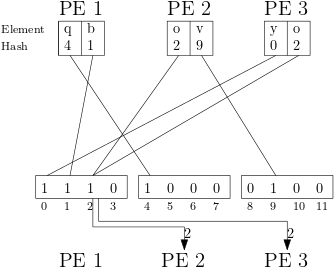
Parallel Bloom filters can be implemented to take advantage of the multiple processing elements (PEs) present in parallel shared-nothing machines. One of the main obstacles for a parallel Bloom filter is the organization and communication of the unordered data which is, in general, distributed evenly over all PEs at the initiation or at batch insertions. To order the data two approaches can be used, either resulting in a Bloom filter over all data being stored on each PE, called replicating bloom filter, or the Bloom filter over all data being split into equal parts, each PE storing one part of it.[31] For both approaches a "Single Shot" Bloom filter is used which only calculates one hash, resulting in one flipped bit per element, to reduce the communication volume.
Distributed Bloom filters are initiated by first hashing all elements on their local PE and then sorting them by their hashes locally. This can be done in linear time using e.g. Bucket sort and also allows local duplicate detection. The sorting is used to group the hashes with their assigned PE as separator to create a Bloom filter for each group. After encoding these Bloom filters using e.g. Golomb coding each bloom filter is send as packet to the PE responsible for the hash values that where inserted into it. A PE p is responsible for all hashes between the values and , where s is the total size of the Bloom filter over all data. Because each element is only hashed once and therefore only a single bit is set, to check if an element was inserted into the Bloom filter only the PE responsible for the hash value of the element needs to be operated on. Single insertion operations can also be done efficiently because the Bloom filter of only one PE has to be changed, compared to Replicating Bloom filters where every PE would have to update its Bloom filter.
By distributing the global Bloom filter over all PEs instead of storing it separately on each PE the Bloom filters size can be far larger, resulting in a larger capacity and lower false positive rate.
Distributed Bloom filters can be used to improve duplicate detection algorithms[32] by filtering out the most 'unique' elements. These can be calculated by communicating only the hashes of elements, not the elements themselves which are far larger in volume, and removing them from the set, reducing the workload for the duplicate detection algorithm used afterwards.
During the communication of the hashes the PEs search for bits that are set in more than one of the receiving packets, as this would mean that two elements had the same hash and therefore could be duplicates. If this occurs a message containing the index of the bit, which is also the hash of the element that could be a duplicate, is send to the PEs which sent a packet with the set bit. If multiple indices are send to the same PE by one sender it can be advantageous to encode the indices as well. All elements that didn't have their hash sent back are now guaranteed to not be a duplicate and won't be evaluated further, for the remaining elements a Repartitioning algorithm[33] can be used. First all the elements that had their hash value sent back are send to the PE that their hash is responsible for. Any element and its duplicate is now guaranteed to be on the same PE. In the second step each PE uses a sequential algorithm for duplicate detection on the receiving elements, which are only a fraction of the amount of starting elements. By allowing a false positive rate for the duplicates, the communication volume can be reduced further as the PEs don't have to send elements with duplicated hashes at all and instead any element with a duplicated hash can simply be marked as a duplicate. As a result the false positive rate for duplicate detection is the same as the false positive rate of the used bloom filter.
The process of filtering out the most 'unique' elements can also be repeated multiple times by changing the hash function in each filtering step. If only a single filtering step is used it has to archive a small false positive rate, however if the filtering step is repeated once the first step can allow a higher false positive rate while the latter one has a higher one but also works on less elements as many have already been removed by the earlier filtering step. While using more than two repetitions can reduce the communication volume further if the number of duplicates in a set is small, the payoff for the additional complications is low.


Replicating Bloom filters organize their data by using a well known hypcercube algorithm for gossiping, e.g. [34]. First each PE calculates the Bloom filter over all local elements and stores it. By repeating a loop where in each step i the PEs send their local Bloom filter over dimension i and merge the Bloom filter they receive over the dimension with their local Bloom filter, it is possible to double the elements each Bloom filter contains in every iteration. After sending and receiving Bloom filters over all dimensions each PE contains the global Bloom filter over all elements.

Replicating Bloom filters are more efficient when the number of queries is much larger than the number of elements that the Bloom filter contains, the break even point compared to Distributed Bloom filters is approximately after accesses, with as the false positive rate of the bloom filter.


Data synchronization
Bloom filters can be used for approximate data synchronization as in Byers et al. (2004). Counting Bloom filters can be used to approximate the number of differences between two sets and this approach is described in Agarwal & Trachtenberg (2006).
Bloomier filters
Chazelle et al. (2004) designed a generalization of Bloom filters that could associate a value with each element that had been inserted, implementing an associative array. Like Bloom filters, these structures achieve a small space overhead by accepting a small probability of false positives. In the case of "Bloomier filters", a false positive is defined as returning a result when the key is not in the map. The map will never return the wrong value for a key that is in the map.
Compact approximators
Boldi & Vigna (2005) proposed a lattice-based generalization of Bloom filters. A compact approximator associates to each key an element of a lattice (the standard Bloom filters being the case of the Boolean two-element lattice). Instead of a bit array, they have an array of lattice elements. When adding a new association between a key and an element of the lattice, they compute the maximum of the current contents of the k array locations associated to the key with the lattice element. When reading the value associated to a key, they compute the minimum of the values found in the k locations associated to the key. The resulting value approximates from above the original value.
Parallel Partitioned Bloom Filters
This implementation used a separate array for each hash function. This method allows for parallel hash calculations for both insertions and inquiries.[35]
Stable Bloom filters
Deng & Rafiei (2006) proposed Stable Bloom filters as a variant of Bloom filters for streaming data. The idea is that since there is no way to store the entire history of a stream (which can be infinite), Stable Bloom filters continuously evict stale information to make room for more recent elements. Since stale information is evicted, the Stable Bloom filter introduces false negatives, which do not appear in traditional Bloom filters. The authors show that a tight upper bound of false positive rates is guaranteed, and the method is superior to standard Bloom filters in terms of false positive rates and time efficiency when a small space and an acceptable false positive rate are given.
Scalable Bloom filters
Almeida et al. (2007) proposed a variant of Bloom filters that can adapt dynamically to the number of elements stored, while assuring a minimum false positive probability. The technique is based on sequences of standard Bloom filters with increasing capacity and tighter false positive probabilities, so as to ensure that a maximum false positive probability can be set beforehand, regardless of the number of elements to be inserted.
Spatial Bloom filters
Spatial Bloom filters (SBF) were originally proposed by Palmieri, Calderoni & Maio (2014) as a data structure designed to store location information, especially in the context of cryptographic protocols for location privacy. However, the main characteristic of SBFs is their ability to store multiple sets in a single data structure, which makes them suitable for a number of different application scenarios.[36] Membership of an element to a specific set can be queried, and the false positive probability depends on the set: the first sets to be entered into the filter during construction have higher false positive probabilities than sets entered at the end.[37] This property allows a prioritization of the sets, where sets containing more "important" elements can be preserved.
Layered Bloom filters
A layered Bloom filter consists of multiple Bloom filter layers. Layered Bloom filters allow keeping track of how many times an item was added to the Bloom filter by checking how many layers contain the item. With a layered Bloom filter a check operation will normally return the deepest layer number the item was found in.[38]
Attenuated Bloom filters
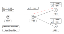
An attenuated Bloom filter of depth D can be viewed as an array of D normal Bloom filters. In the context of service discovery in a network, each node stores regular and attenuated Bloom filters locally. The regular or local Bloom filter indicates which services are offered by the node itself. The attenuated filter of level i indicates which services can be found on nodes that are i-hops away from the current node. The i-th value is constructed by taking a union of local Bloom filters for nodes i-hops away from the node.[39]
Let's take a small network shown on the graph below as an example. Say we are searching for a service A whose id hashes to bits 0,1, and 3 (pattern 11010). Let n1 node to be the starting point. First, we check whether service A is offered by n1 by checking its local filter. Since the patterns don't match, we check the attenuated Bloom filter in order to determine which node should be the next hop. We see that n2 doesn't offer service A but lies on the path to nodes that do. Hence, we move to n2 and repeat the same procedure. We quickly find that n3 offers the service, and hence the destination is located.[40]
By using attenuated Bloom filters consisting of multiple layers, services at more than one hop distance can be discovered while avoiding saturation of the Bloom filter by attenuating (shifting out) bits set by sources further away.[39]
Chemical structure searching
Bloom filters are often used to search large chemical structure databases (see chemical similarity). In the simplest case, the elements added to the filter (called a fingerprint in this field) are just the atomic numbers present in the molecule, or a hash based on the atomic number of each atom and the number and type of its bonds. This case is too simple to be useful. More advanced filters also encode atom counts, larger substructure features like carboxyl groups, and graph properties like the number of rings. In hash-based fingerprints, a hash function based on atom and bond properties is used to turn a subgraph into a PRNG seed, and the first output values used to set bits in the Bloom filter.
Molecular fingerprints started in the late 1940s as way to search for chemical structures searched on punched cards. However, it wasn't until around 1990 that Daylight Chemical Information Systems, Inc. introduced a hash-based method to generate the bits, rather than use a precomputed table. Unlike the dictionary approach, the hash method can assign bits for substructures which hadn't previously been seen. In the early 1990s, the term "fingerprint" was considered different from "structural keys", but the term has since grown to encompass most molecular characteristics which can be used for a similarity comparison, including structural keys, sparse count fingerprints, and 3D fingerprints. Unlike Bloom filters, the Daylight hash method allows the number of bits assigned per feature to be a function of the feature size, but most implementations of Daylight-like fingerprints use a fixed number of bits per feature, which makes them a Bloom filter. The original Daylight fingerprints could be used for both similarity and screening purposes. Many other fingerprint types, like the popular ECFP2, can be used for similarity but not for screening because they include local environmental characteristics that introduce false negatives when used as a screen. Even if these are constructed with the same mechanism, these are not Bloom filters because they cannot be used to filter.
See also
Notes
- Bloom (1970).
- Bonomi et al. (2006).
- Dillinger & Manolios (2004a); Kirsch & Mitzenmacher (2006).
- Mitzenmacher & Upfal (2005).
- Blustein & El-Maazawi (2002), pp. 21–22
- Mitzenmacher & Upfal (2005), pp. 109–111, 308.
- Mitzenmacher & Upfal (2005), p. 308.
- Starobinski, Trachtenberg & Agarwal (2003)
- Goel & Gupta (2010)
- Dasgupta, Sanjoy; Sheehan, Timothy C.; Stevens, Charles F.; Navlakha, Saket (2018-12-18). "A neural data structure for novelty detection". Proceedings of the National Academy of Sciences. 115 (51): 13093–13098. doi:10.1073/pnas.1814448115. ISSN 0027-8424. PMC 6304992. PMID 30509984.
- Maggs & Sitaraman (2015).
- "Bloom index contrib module". Postgresql.org. 2016-04-01. Archived from the original on 2018-09-09. Retrieved 2016-06-18.
- Chang et al. (2006); Apache Software Foundation (2012).
- Yakunin, Alex (2010-03-25). "Alex Yakunin's blog: Nice Bloom filter application". Blog.alexyakunin.com. Archived from the original on 2010-10-27. Retrieved 2014-05-31.
- "Issue 10896048: Transition safe browsing from bloom filter to prefix set. - Code Review". Chromiumcodereview.appspot.com. Retrieved 2014-07-03.
- Goodwin, Bob; Hopcroft, Michael; Luu, Dan; Clemmer, Alex; Curmei, Mihaela; Elnikety, Sameh; Yuxiong, He (2017). "BitFunnel: Revisiting Signatures for Search" (PDF). SIGIR: 605–614. doi:10.1145/3077136.3080789.
- Wessels (2004).
- "BIP 0037". 2012-10-24. Retrieved 2018-05-29.
- "Plan 9 /sys/man/8/venti". Plan9.bell-labs.com. Archived from the original on 2014-08-28. Retrieved 2014-05-31.
- "Spin - Formal Verification".
- Mullin (1990).
- "Exim source code". github. Retrieved 2014-03-03.
- "What are Bloom filters?". Medium. 2015-07-15. Retrieved 2015-11-01.
- Pagh, Pagh & Rao (2005).
- Luo, Lailong; Guo, Deke; Ma, Richard T.B.; Rottenstreich, Ori; Luo, Xueshan (13 Apr 2018). "Optimizing Bloom filter: Challenges, solutions, and comparisons". arXiv:1804.04777 [cs.DS].
- Luo, Lailong; Guo, Deke; Ma, Richard T.B.; Rottenstreich, Ori; Luo, Xueshan (13 Apr 2018). "Optimizing Bloom filter: Challenges, solutions, and comparisons". arXiv:1804.04777 [cs.DS].
- Dasgupta, Sanjoy; Sheehan, Timothy C.; Stevens, Charles F.; Navlakhae, Saket (2018). "A neural data structure for novelty detection". Proceedings of the National Academy of Sciences. 115 (51): 13093–13098. doi:10.1073/pnas.1814448115. PMC 6304992. PMID 30509984.
- Kiss, S. Z.; Hosszu, E.; Tapolcai, J.; Rónyai, L.; Rottenstreich, O. (2018). "Bloom filter with a false positive free zone" (PDF). IEEE Proceedings of INFOCOM. Retrieved 4 December 2018.
- Kim, Kibeom; Jeong, Yongjo; Lee, Youngjoo; Lee, Sunggu (2019-07-11). "Analysis of Counting Bloom Filters Used for Count Thresholding". Electronics. 8 (7): 779. doi:10.3390/electronics8070779. ISSN 2079-9292.
- Pournaras, Warnier & Brazier (2013).
- Sanders, Peter and Schlag, Sebastian and Müller, Ingo (2013). "Communication efficient algorithms for fundamental big data problems". 2013 IEEE International Conference on Big Data: 15–23.CS1 maint: multiple names: authors list (link)
- Schlag, Sebastian (2013). "Distributed duplicate removal". Karlsruhe Institute of Technology.
- Shatdal, Ambuj, and Jeffrey F. Naughton (1994). "Processing aggregates in parallel database systems". University of Wisconsin-Madison Department of Computer Sciences: 8.CS1 maint: multiple names: authors list (link)
- V. Kumar, A. Grama, A. Gupta, and G. Karypis (1994). Introduction to Parallel Computing. Design and Analysis of Algorithms. Benjamin/Cummings.CS1 maint: multiple names: authors list (link)
- Kirsch, Adam; Mitzenmacher†, Michael. "Less Hashing, Same Performance: Building a Better Bloom Filter" (PDF). Harvard School of Engineering and Applied Sciences. Wiley InterScience.
- Calderoni, Palmieri & Maio (2015).
- Calderoni, Palmieri & Maio (2018).
- Zhiwang, Jungang & Jian (2010).
- Koucheryavy et al. (2009).
- Kubiatowicz et al. (2000).
References
- Agarwal, Sachin; Trachtenberg, Ari (2006), "Approximating the number of differences between remote sets" (PDF), IEEE Information Theory Workshop, Punta del Este, Uruguay: 217, CiteSeerX 10.1.1.69.1033, doi:10.1109/ITW.2006.1633815, ISBN 978-1-4244-0035-5
- Ahmadi, Mahmood; Wong, Stephan (2007), "A Cache Architecture for Counting Bloom Filters", 15th international Conference on Networks (ICON-2007), p. 218, CiteSeerX 10.1.1.125.2470, doi:10.1109/ICON.2007.4444089, ISBN 978-1-4244-1229-7
- Almeida, Paulo; Baquero, Carlos; Preguica, Nuno; Hutchison, David (2007), "Scalable Bloom Filters" (PDF), Information Processing Letters, 101 (6): 255–261, doi:10.1016/j.ipl.2006.10.007, hdl:1822/6627
- Apache Software Foundation (2012), "11.6. Schema Design", The Apache HBase Reference Guide, Revision 0.94.27
- Bloom, Burton H. (1970), "Space/Time Trade-offs in Hash Coding with Allowable Errors", Communications of the ACM, 13 (7): 422–426, CiteSeerX 10.1.1.641.9096, doi:10.1145/362686.362692
- Blustein, James; El-Maazawi, Amal (2002), "optimal case for general Bloom filters", Bloom Filters — A Tutorial, Analysis, and Survey, Dalhousie University Faculty of Computer Science, pp. 1–31
- Boldi, Paolo; Vigna, Sebastiano (2005), "Mutable strings in Java: design, implementation and lightweight text-search algorithms", Science of Computer Programming, 54 (1): 3–23, doi:10.1016/j.scico.2004.05.003
- Bonomi, Flavio; Mitzenmacher, Michael; Panigrahy, Rina; Singh, Sushil; Varghese, George (2006), "An Improved Construction for Counting Bloom Filters", Algorithms – ESA 2006, 14th Annual European Symposium (PDF), Lecture Notes in Computer Science, 4168, pp. 684–695, doi:10.1007/11841036_61, ISBN 978-3-540-38875-3
- Broder, Andrei; Mitzenmacher, Michael (2005), "Network Applications of Bloom Filters: A Survey" (PDF), Internet Mathematics, 1 (4): 485–509, doi:10.1080/15427951.2004.10129096
- Byers, John W.; Considine, Jeffrey; Mitzenmacher, Michael; Rost, Stanislav (2004), "Informed content delivery across adaptive overlay networks", IEEE/ACM Transactions on Networking, 12 (5): 767, CiteSeerX 10.1.1.207.1563, doi:10.1109/TNET.2004.836103
- Calderoni, Luca; Palmieri, Paolo; Maio, Dario (2015), "Location privacy without mutual trust: The spatial Bloom filter" (PDF), Computer Communications, 68: 4–16, doi:10.1016/j.comcom.2015.06.011, hdl:10468/4762, ISSN 0140-3664
- Calderoni, Luca; Palmieri, Paolo; Maio, Dario (2018), "Probabilistic Properties of the Spatial Bloom Filters and Their Relevance to Cryptographic Protocols", IEEE Transactions on Information Forensics and Security, 13 (7): 1710–1721, doi:10.1109/TIFS.2018.2799486, hdl:10468/5767, ISSN 1556-6013*Chang, Fay; Dean, Jeffrey; Ghemawat, Sanjay; Hsieh, Wilson; Wallach, Deborah; Burrows, Mike; Chandra, Tushar; Fikes, Andrew; Gruber, Robert (2006), "Bigtable: A Distributed Storage System for Structured Data", Seventh Symposium on Operating System Design and Implementation
- Charles, Denis Xavier; Chellapilla, Kumar (2008), "Bloomier filters: A second look", in Halperin, Dan; Mehlhorn, Kurt (eds.), Algorithms: ESA 2008, 16th Annual European Symposium, Karlsruhe, Germany, September 15–17, 2008, Proceedings, Lecture Notes in Computer Science, 5193, Springer, pp. 259–270, arXiv:0807.0928, doi:10.1007/978-3-540-87744-8_22, ISBN 978-3-540-87743-1
- Chazelle, Bernard; Kilian, Joe; Rubinfeld, Ronitt; Tal, Ayellet (2004), "The Bloomier filter: an efficient data structure for static support lookup tables", Proceedings of the Fifteenth Annual ACM-SIAM Symposium on Discrete Algorithms (PDF), pp. 30–39
- Cohen, Saar; Matias, Yossi (2003), "Spectral Bloom Filters", Proceedings of the 2003 ACM SIGMOD International Conference on Management of Data (PDF), pp. 241–252, doi:10.1145/872757.872787, ISBN 978-1581136340
- Deng, Fan; Rafiei, Davood (2006), "Approximately Detecting Duplicates for Streaming Data using Stable Bloom Filters", Proceedings of the ACM SIGMOD Conference (PDF), pp. 25–36
- Dharmapurikar, Sarang; Song, Haoyu; Turner, Jonathan; Lockwood, John (2006), "Fast packet classification using Bloom filters", Proceedings of the 2006 ACM/IEEE Symposium on Architecture for Networking and Communications Systems (PDF), pp. 61–70, CiteSeerX 10.1.1.78.9584, doi:10.1145/1185347.1185356, ISBN 978-1595935809, archived from the original (PDF) on 2007-02-02
- Dietzfelbinger, Martin; Pagh, Rasmus (2008), "Succinct data structures for retrieval and approximate membership", in Aceto, Luca; Damgård, Ivan; Goldberg, Leslie Ann; Halldórsson, Magnús M.; Ingólfsdóttir, Anna; Walukiewicz, Igor (eds.), Automata, Languages and Programming: 35th International Colloquium, ICALP 2008, Reykjavik, Iceland, July 7–11, 2008, Proceedings, Part I, Track A: Algorithms, Automata, Complexity, and Games, Lecture Notes in Computer Science, 5125, Springer, pp. 385–396, arXiv:0803.3693, doi:10.1007/978-3-540-70575-8_32, ISBN 978-3-540-70574-1
- Dillinger, Peter C.; Manolios, Panagiotis (2004a), "Fast and Accurate Bitstate Verification for SPIN", Proceedings of the 11th International Spin Workshop on Model Checking Software, Springer-Verlag, Lecture Notes in Computer Science 2989
- Dillinger, Peter C.; Manolios, Panagiotis (2004b), "Bloom Filters in Probabilistic Verification", Proceedings of the 5th International Conference on Formal Methods in Computer-Aided Design, Springer-Verlag, Lecture Notes in Computer Science 3312
- Donnet, Benoit; Baynat, Bruno; Friedman, Timur (2006), "Retouched Bloom Filters: Allowing Networked Applications to Flexibly Trade Off False Positives Against False Negatives", CoNEXT 06 – 2nd Conference on Future Networking Technologies, archived from the original on 2009-05-17
- Eppstein, David; Goodrich, Michael T. (2007), "Space-efficient straggler identification in round-trip data streams via Newton's identities and invertible Bloom filters", Algorithms and Data Structures, 10th International Workshop, WADS 2007, Lecture Notes in Computer Science, 4619, Springer-Verlag, pp. 637–648, arXiv:0704.3313, Bibcode:2007arXiv0704.3313E
- Fan, Bin; Andersen, Dave G.; Kaminsky, Michael; Mitzenmacher, Michael D. (2014), "Cuckoo filter: Practically better than Bloom", Proc. 10th ACM Int. Conf. Emerging Networking Experiments and Technologies (CoNEXT '14), pp. 75–88, doi:10.1145/2674005.2674994, ISBN 9781450332798. Open source implementation available on github.
- Fan, Li; Cao, Pei; Almeida, Jussara; Broder, Andrei (2000), "Summary Cache: A Scalable Wide-Area Web Cache Sharing Protocol" (PDF), IEEE/ACM Transactions on Networking, 8 (3): 281–293, CiteSeerX 10.1.1.41.1487, doi:10.1109/90.851975. A preliminary version appeared at SIGCOMM '98.
- Goel, Ashish; Gupta, Pankaj (2010), "Small subset queries and bloom filters using ternary associative memories, with applications" (PDF), ACM Sigmetrics 2010, 38: 143, CiteSeerX 10.1.1.296.6513, doi:10.1145/1811099.1811056
- Graf, Thomas Mueller; Lemire, Daniel (2019), Xor Filters: Faster and Smaller Than Bloom and Cuckoo Filters, arXiv:1912.08258, Bibcode:2019arXiv191208258M
- Grandi, Fabio (2018), "On the analysis of Bloom filters" (PDF), Information Processing Letters, 129: 35–39, doi:10.1016/j.ipl.2017.09.004
- Kirsch, Adam; Mitzenmacher, Michael (2006), "Less Hashing, Same Performance: Building a Better Bloom Filter", in Azar, Yossi; Erlebach, Thomas (eds.), Algorithms – ESA 2006, 14th Annual European Symposium (PDF), Lecture Notes in Computer Science, 4168, Springer-Verlag, Lecture Notes in Computer Science 4168, pp. 456–467, doi:10.1007/11841036, ISBN 978-3-540-38875-3, archived from the original (PDF) on 2009-01-31
- Koucheryavy, Y.; Giambene, G.; Staehle, D.; Barcelo-Arroyo, F.; Braun, T.; Siris, V. (2009), "Traffic and QoS Management in Wireless Multimedia Networks", COST 290 Final Report: 111
- Kubiatowicz, J.; Bindel, D.; Czerwinski, Y.; Geels, S.; Eaton, D.; Gummadi, R.; Rhea, S.; Weatherspoon, H.; et al. (2000), "Oceanstore: An architecture for global-scale persistent storage" (PDF), ACM SIGPLAN Notices: 190–201, archived from the original (PDF) on 2012-03-11, retrieved 2011-12-01
- Maggs, Bruce M.; Sitaraman, Ramesh K. (July 2015), "Algorithmic nuggets in content delivery" (PDF), SIGCOMM Computer Communication Review, 45 (3): 52–66, CiteSeerX 10.1.1.696.9236, doi:10.1145/2805789.2805800
- Mitzenmacher, Michael; Upfal, Eli (2005), Probability and computing: Randomized algorithms and probabilistic analysis, Cambridge University Press, pp. 107–112, ISBN 9780521835404
- Mortensen, Christian Worm; Pagh, Rasmus; Pătraşcu, Mihai (2005), "On dynamic range reporting in one dimension", Proceedings of the Thirty-seventh Annual ACM Symposium on Theory of Computing, pp. 104–111, arXiv:cs/0502032, doi:10.1145/1060590.1060606, ISBN 978-1581139600
- Mullin, James K. (1990), "Optimal semijoins for distributed database systems", IEEE Transactions on Software Engineering, 16 (5): 558–560, doi:10.1109/32.52778
- Pagh, Anna; Pagh, Rasmus; Rao, S. Srinivasa (2005), "An optimal Bloom filter replacement", Proceedings of the Sixteenth Annual ACM-SIAM Symposium on Discrete Algorithms (PDF), pp. 823–829
- Palmieri, Paolo; Calderoni, Luca; Maio, Dario (2014), "Spatial Bloom Filters: Enabling Privacy in Location-Aware Applications", Proc. 10th International Conference on Information Security and Cryptology (Inscrypt 2014), 8957, Springer-Verlag, Lecture Notes in Computer Science, pp. 16–36, CiteSeerX 10.1.1.471.4759, doi:10.1007/978-3-319-16745-9_2, ISBN 978-3-319-16744-2
- Porat, Ely (2009), "An optimal Bloom filter replacement based on matrix solving", in Frid, Anna E.; Morozov, Andrey; Rybalchenko, Andrey; Wagner, Klaus W. (eds.), Computer Science, Theory and Applications: Fourth International Computer Science Symposium in Russia, CSR 2009, Novosibirsk, Russia, August 18–23, 2009, Proceedings, Lecture Notes in Computer Science, 5675, Springer, pp. 263–273, arXiv:0804.1845, doi:10.1007/978-3-642-03351-3_25, ISBN 978-3-642-03350-6
- Pournaras, E.; Warnier, M.; Brazier, F.M.T.. (2013), "A generic and adaptive aggregation service for large-scale decentralized networks", Complex Adaptive Systems Modeling, 1:19: 19, doi:10.1186/2194-3206-1-19. Prototype implementation available on github.
- Putze, F.; Sanders, P.; Singler, J. (2007), "Cache-, Hash- and Space-Efficient Bloom Filters", in Demetrescu, Camil (ed.), Experimental Algorithms, 6th International Workshop, WEA 2007 (PDF), Lecture Notes in Computer Science, 4525, Springer-Verlag, Lecture Notes in Computer Science 4525, pp. 108–121, doi:10.1007/978-3-540-72845-0, ISBN 978-3-540-72844-3
- Rottenstreich, Ori; Kanizo, Yossi; Keslassy, Isaac (2012), "The Variable-Increment Counting Bloom Filter", 31st Annual IEEE International Conference on Computer Communications, 2012, Infocom 2012 (PDF), pp. 1880–1888, CiteSeerX 10.1.1.174.7165, doi:10.1109/INFCOM.2012.6195563, ISBN 978-1-4673-0773-4
- Sethumadhavan, Simha; Desikan, Rajagopalan; Burger, Doug; Moore, Charles R.; Keckler, Stephen W. (2003), "Scalable hardware memory disambiguation for high ILP processors", 36th Annual IEEE/ACM International Symposium on Microarchitecture, 2003, MICRO-36 (PDF), pp. 399–410, CiteSeerX 10.1.1.229.1254, doi:10.1109/MICRO.2003.1253244, ISBN 978-0-7695-2043-8, archived from the original (PDF) on 2007-01-14
- Starobinski, David; Trachtenberg, Ari; Agarwal, Sachin (2003), "Efficient PDA Synchronization" (PDF), IEEE Transactions on Mobile Computing, 2 (1): 40, CiteSeerX 10.1.1.71.7833, doi:10.1109/TMC.2003.1195150
- Stern, Ulrich; Dill, David L. (1996), "A New Scheme for Memory-Efficient Probabilistic Verification", Proceedings of Formal Description Techniques for Distributed Systems and Communication Protocols, and Protocol Specification, Testing, and Verification: IFIP TC6/WG6.1 Joint International Conference, Chapman & Hall, IFIP Conference Proceedings, pp. 333–348, CiteSeerX 10.1.1.47.4101
- Swamidass, S. Joshua; Baldi, Pierre (2007), "Mathematical correction for fingerprint similarity measures to improve chemical retrieval", Journal of Chemical Information and Modeling, 47 (3): 952–964, doi:10.1021/ci600526a, PMID 17444629
- Wessels, Duane (January 2004), "10.7 Cache Digests", Squid: The Definitive Guide (1st ed.), O'Reilly Media, p. 172, ISBN 978-0-596-00162-9,
Cache Digests are based on a technique first published by Pei Cao, called Summary Cache. The fundamental idea is to use a Bloom filter to represent the cache contents.
- Tarkoma, Sasu; Rothenberg, Christian Esteve; Lagerspetz, Eemil (2012), "Theory and practice of bloom filters for distributed systems", IEEE Communications Surveys & Tutorials, no. 1. (PDF), 14, pp. 131–155
- Zhiwang, Cen; Jungang, Xu; Jian, Sun (2010), "A multi-layer Bloom filter for duplicated URL detection", Proc. 3rd International Conference on Advanced Computer Theory and Engineering (ICACTE 2010), 1, pp. V1–586–V1–591, doi:10.1109/ICACTE.2010.5578947, ISBN 978-1-4244-6539-2
External links
| Wikimedia Commons has media related to Bloom filter. |
- "Using Bloom Filters" Detailed Bloom Filter explanation using Perl
- Why Bloom filters work the way they do (Michael Nielsen, 2012)
- Bloom Filters — A Tutorial, Analysis, and Survey (Blustein & El-Maazawi, 2002) at Dalhousie University
- Table of false-positive rates for different configurations from a University of Wisconsin–Madison website
- "More Optimal Bloom Filters," Ely Porat (Nov/2007) Google TechTalk video on YouTube