Backward differentiation formula
The backward differentiation formula (BDF) is a family of implicit methods for the numerical integration of ordinary differential equations. They are linear multistep methods that, for a given function and time, approximate the derivative of that function using information from already computed time points, thereby increasing the accuracy of the approximation. These methods are especially used for the solution of stiff differential equations. The methods were first introduced by Charles F. Curtiss and Joseph O. Hirschfelder in 1952.[1]
General formula
A BDF is used to solve the initial value problem

The general formula for a BDF can be written as [2]

where denotes the step size and . Since is evaluated for the unknown , BDF methods are implicit and possibly require the solution of nonlinear equations at each step. The coefficients and are chosen so that the method achieves order , which is the maximum possible.


Derivation of the coefficients
Starting from the formula one approximates and , where is the Lagrange interpolation polynomial for the points . Using that and multiplying by one arrives at the BDF method of order .


Specific formulas
The s-step BDFs with s < 7 are:[3]
- BDF1: (this is the backward Euler method)
- BDF2:
- BDF3:
- BDF4:
- BDF5:
- BDF6:


Methods with s > 6 are not zero-stable so they cannot be used.[4]
Stability
The stability of numerical methods for solving stiff equations is indicated by their region of absolute stability. For the BDF methods, these regions are shown in the plots below.
Ideally, the region contains the left half of the complex plane, in which case the method is said to be A-stable. However, linear multistep methods with an order greater than 2 cannot be A-stable. The stability region of the higher-order BDF methods contain a large part of the left half-plane and in particular the whole of the negative real axis. The BDF methods are the most efficient linear multistep methods of this kind.[4]
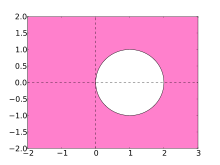 BDF1
BDF1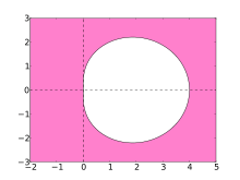 BDF2
BDF2 BDF3
BDF3 BDF4
BDF4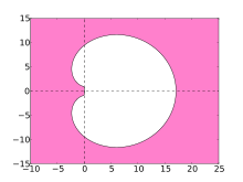 BDF5
BDF5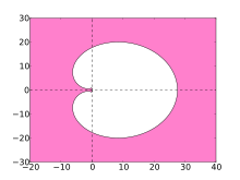 BDF6
BDF6
References
Citations
- Curtiss, C. F., & Hirschfelder, J. O. (1952). Integration of stiff equations. Proceedings of the National Academy of Sciences, 38(3), 235-243.
- Ascher & Petzold 1998, §5.1.2, p. 129
- Iserles 1996, p. 27 (for s = 1, 2, 3); Süli & Mayers 2003, p. 349 (for all s)
- Süli & Mayers 2003, p. 349
Referred works
- Ascher, U. M.; Petzold, L. R. (1998), Computer Methods for Ordinary Differential Equations and Differential-Algebraic Equations, SIAM, Philadelphia, ISBN 0-89871-412-5.
- Iserles, Arieh (1996), A First Course in the Numerical Analysis of Differential Equations, Cambridge University Press, ISBN 978-0-521-55655-2.
- Süli, Endre; Mayers, David (2003), An Introduction to Numerical Analysis, Cambridge University Press, ISBN 0-521-00794-1.
Further reading
- BDF Methods at the SUNDIALS wiki (SUNDIALS is a library implementing BDF methods and similar algorithms).