Arrhenius plot
In chemical kinetics, an Arrhenius plot displays the logarithm of a reaction rate constant, (, ordinate axis) plotted against reciprocal of the temperature (, abscissa). Arrhenius plots are often used to analyze the effect of temperature on the rates of chemical reactions. For a single rate-limited thermally activated process, an Arrhenius plot gives a straight line, from which the activation energy and the pre-exponential factor can both be determined.


The Arrhenius equation can be given in the form: that

Where:
- = Rate constant
- = Pre-exponential factor
- = Activation energy
- = Boltzmann constant
- = Gas constant, equivalent to times Avogadro's constant.
- = Absolute temperature, K


The only difference is the energy units: the former form uses energy/mole, which is common in chemistry, while the latter form uses energy on the scale of individual particles directly, which is common in physics. The different units are accounted for in using either the gas constant or the Boltzmann constant .
Taking the natural logarithm of the former equation gives.

When plotted in the manner described above, the value of the y-intercept (at ) will correspond to , and the slope of the line will be equal to . The values of y-intercept and slope can be determined from the experimental points using simple linear regression with a spreadsheet.


The pre-exponential factor, A, is an empirical constant of proportionality which has been estimated by various theories which take into account factors such as the frequency of collision between reacting particles, their relative orientation, and the entropy of activation.
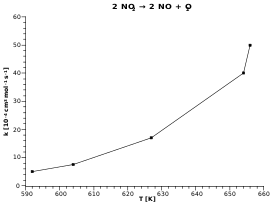
The expression represents the fraction of the molecules present in a gas which have energies equal to or in excess of activation energy at a particular temperature. In almost all practical cases, , so that this fraction is very small and increases rapidly with T. In consequence, the reaction rate constant k increases rapidly with temperature T, as shown in the direct plot of k against T. (Mathematically, at very high temperatures so that , k would level off and approach A as a limit, but this case does not occur under practical conditions.)


Worked example
This example uses the decay of nitrogen dioxide: 2 NO2 → 2 NO + O2
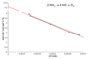
Based on the red "line of best fit" plotted in the graph given above:
- Let y = ln(k[10−4 cm3 mol−1 s−1])
- Let x = 1/T[K]
Points read from graph:
- y = 4.1 at x = 0.0015
- y = 2.2 at x = 0.00165
Slope of red line = (4.1 - 2.2) / (0.0015 - 0.00165) = -12,667
Intercept [y-value at x=0] of red line = 4.1 + (0.0015 x 12667) = 23.1
Inserting these values into the form above:
yields:


as shown in the plot at the right.

for:
- k in 10−4 cm3 mol−1 s−1
- T in K
Substituting for the quotient in the exponent of :

- -Ea / R = -12,667 K
- approximate value for R = 8.31446 J K−1 mol−1
The activation energy of this reaction from these data is then:
- Ea = R x 12,667 K = 105,300 J mol−1 = 105.3 kJ mol−1.