Y-Δ transform

The Y-Δ transform, also written wye-delta and also known by many other names, is a mathematical technique to simplify the analysis of an electrical network. The name derives from the shapes of the circuit diagrams, which look respectively like the letter Y and the Greek capital letter Δ. This circuit transformation theory was published by Arthur Edwin Kennelly in 1899.^[1] It is widely used in analysis of three-phase electric power circuits.

The Y-Δ transform can be considered a special case of the star-mesh transform for three resistors. In mathematics, the Y-Δ transform plays an important role in theory of circular planar graphs.^[2]

Names

Illustration of the transform in its T-Π representation.

The Y-Δ transform is known by a variety of other names, mostly based upon the two shapes involved, listed in either order. The Y, spelled out as wye, can also be called T or star; the Δ, spelled out as delta, can also be called triangle, Π (spelled out as pi), or mesh. Thus, common names for the transformation include wye-delta or delta-wye, star-delta, star-mesh, or T-Π.

Basic Y-Δ transformation

Δ and Y circuits with the labels which are used in this article.

The transformation is used to establish equivalence for networks with three terminals. Where three elements terminate at a common node and none are sources, the node is eliminated by transforming the impedances. For equivalence, the impedance between any pair of terminals must be the same for both networks. The equations given here are valid for complex as well as real impedances.

Equations for the transformation from Δ to Y

The general idea is to compute the impedance $R_{Y}$ at a terminal node of the Y circuit with impedances $R'$ , $R''$ to adjacent nodes in the Δ circuit by

R_{Y}={\frac {R'R''}{\sum R_{\Delta }}}

where $R_\Delta$ are all impedances in the Δ circuit. This yields the specific formulae

\begin{align} R_1 &= \frac{R_bR_c}{R_a + R_b + R_c} \\ R_2 &= \frac{R_aR_c}{R_a + R_b + R_c} \\ R_3 &= \frac{R_aR_b}{R_a + R_b + R_c} \end{align}

Equations for the transformation from Y to Δ

The general idea is to compute an impedance $R_\Delta$ in the Δ circuit by

R_\Delta = \frac{R_P}{R_\mathrm{opposite}}

where $R_P = R_1R_2+R_2R_3+R_3R_1$ is the sum of the products of all pairs of impedances in the Y circuit and $R_\mathrm{opposite}$ is the impedance of the node in the Y circuit which is opposite the edge with $R_\Delta$ . The formula for the individual edges are thus

\begin{align} R_a &= \frac{R_1R_2 + R_2R_3 + R_3R_1}{R_1} \\ R_b &= \frac{R_1R_2 + R_2R_3 + R_3R_1}{R_2} \\ R_c &= \frac{R_1R_2 + R_2R_3 + R_3R_1}{R_3} \end{align}

Or, if using admittance instead of resistance:

{\begin{aligned}Y_{a}={\frac {Y_{3}Y_{2}}{\sum Y_{Y}}}\\Y_{b}={\frac {Y_{3}Y_{1}}{\sum Y_{Y}}}\\Y_{c}={\frac {Y_{1}Y_{2}}{\sum Y_{Y}}}\end{aligned}}

Note that the general formula in Y to Δ using admittance is similar to Δ to Y using resistance.

A proof of the existence and uniqueness of the transformation

The feasibility of the transformation can be shown as a consequence of the superposition theorem for electric circuits. A short proof, rather than one derived as a corollary of the more general star-mesh transform, can be given as follows. The equivalence lies in the statement that for any external voltages ( $V_{1},V_{2}$ and $V_{3}$ ) applying at the three nodes ( $N_{1},N_{2}$ and $N_3$ ), the corresponding currents ( $I_{1},I_{2}$ and $I_{3}$ ) are exactly the same for both the Y and Δ circuit, and vice versa. In this proof, we start with given external currents at the nodes. According to the superposition theorem, the voltages can be obtained by studying the superposition of the resulting voltages at the nodes of the following three problems applied at the three nodes with current:

${\frac {1}{3}}\left(I_{1}-I_{2}\right),-{\frac {1}{3}}\left(I_{1}-I_{2}\right),0$
$0,{\frac {1}{3}}\left(I_{2}-I_{3}\right),-{\frac {1}{3}}\left(I_{2}-I_{3}\right)$ and
$-{\frac {1}{3}}\left(I_{3}-I_{1}\right),0,{\frac {1}{3}}\left(I_{3}-I_{1}\right)$

The equivalence can be readily shown by using Kirchhoff's circuit laws that $I_{1}+I_{2}+I_{3}=0$ . Now each problem is relatively simple, since it involves only one single ideal current source. To obtain exactly the same outcome voltages at the nodes for each problem, the equivalent resistances in the two circuits must be the same, this can be easily found by using the basic rules of series and parallel circuits:

R_{3}+R_{1}={\frac {\left(R_{c}+R_{a}\right)R_{b}}{R_{a}+R_{b}+R_{c}}},\quad {\frac {R_{3}}{R_{1}}}={\frac {R_{a}}{R_{c}}}.

Though usually six equations are more than enough to express three variables ( $R_{1},R_{2},R_{3}$ ) in term of the other three variables( $R_{a},R_{b},R_{c}$ ), here it is straightforward to show that these equations indeed lead to the above designed expressions.

In fact, the superposition theorem establishes the relation between the values of the resistances, the uniqueness theorem guarantees the uniqueness of such solution.

Simplification of networks

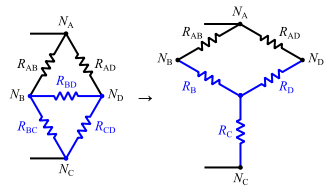
Resistive networks between two terminals can theoretically be simplified to a single equivalent resistor (more generally, the same is true of impedance). Series and parallel transforms are basic tools for doing so, but for complex networks such as the bridge illustrated here, they do not suffice.

The Y-Δ transform can be used to eliminate one node at a time and produce a network that can be further simplified, as shown.

Transformation of a bridge resistor network, using the Y-Δ transform to eliminate node D, yields an equivalent network that may readily be simplified further.

The reverse transformation, Δ-Y, which adds a node, is often handy to pave the way for further simplification as well.

Transformation of a bridge resistor network, using the Δ-Y transform, also yields an equivalent network that may readily be simplified further.

Every two-terminal network represented by a planar graph can be reduced to a single equivalent resistor by a sequence of series, parallel, Y-Δ, and Δ-Y transformations.^[3] However, there are non-planar networks that cannot be simplified using these transformations, such as a regular square grid wrapped around a torus, or any member of the Petersen family.

Graph theory

In graph theory, the Y-Δ transform means replacing a Y subgraph of a graph with the equivalent Δ subgraph. The transform preserves the number of edges in a graph, but not the number of vertices or the number of cycles. Two graphs are said to be Y-Δ equivalent if one can be obtained from the other by a series of Y-Δ transforms in either direction. For example, the Petersen family is a Y-Δ equivalence class.

Demonstration

Δ-load to Y-load transformation equations

Δ and Y circuits with the labels that are used in this article.

To relate $\{R_a, R_b, R_c\}$ from Δ to $\{R_1,R_2,R_3\}$ from Y, the impedance between two corresponding nodes is compared. The impedance in either configuration is determined as if one of the nodes is disconnected from the circuit.

The impedance between N₁ and N₂ with N₃ disconnected in Δ:

\begin{align} R_\Delta(N_1, N_2) &= R_c \parallel (R_a + R_b) \\ &= \frac{1}{\frac{1}{R_c} + \frac{1}{R_a + R_b}} \\ &= \frac{R_c(R_a + R_b)}{R_a + R_b + R_c} \end{align}

To simplify, let $R_T$ be the sum of $\{R_a, R_b, R_c\}$ .

R_T = R_a + R_b + R_c

Thus,

R_\Delta(N_1, N_2) = \frac{R_c(R_a+R_b)}{R_T}

The corresponding impedance between N₁ and N₂ in Y is simple:

R_Y(N_1, N_2) = R_1 + R_2

hence:

R_1+R_2 = \frac{R_c(R_a+R_b)}{R_T}

(1)

Repeating for $R(N_2,N_3)$ :

R_2+R_3 = \frac{R_a(R_b+R_c)}{R_T}

(2)

and for $R(N_1,N_3)$ :

R_1+R_3 = \frac{R_b(R_a+R_c)}{R_T}.

(3)

From here, the values of $\{R_1,R_2,R_3\}$ can be determined by linear combination (addition and/or subtraction).

For example, adding (1) and (3), then subtracting (2) yields

R_1+R_2+R_1+R_3-R_2-R_3 = \frac{R_c(R_a+R_b)}{R_T} + \frac{R_b(R_a+R_c)}{R_T} - \frac{R_a(R_b+R_c)}{R_T}

2R_1 = \frac{2R_bR_c}{R_T}

thus,

R_1 = \frac{R_bR_c}{R_T}.

where $R_T = R_a + R_b + R_c$

For completeness:

R_1 = \frac{R_bR_c}{R_T}

(4)

R_2 = \frac{R_aR_c}{R_T}

(5)

R_3 = \frac{R_aR_b}{R_T}

(6)

Y-load to Δ-load transformation equations

Let

R_T = R_a+R_b+R_c

.

We can write the Δ to Y equations as

R_1 = \frac{R_bR_c}{R_T}

(1)

R_2 = \frac{R_aR_c}{R_T}

(2)

R_3 = \frac{R_aR_b}{R_T}.

(3)

Multiplying the pairs of equations yields

R_1R_2 = \frac{R_aR_bR_c^2}{R_T^2}

(4)

R_1R_3 = \frac{R_aR_b^2R_c}{R_T^2}

(5)

R_2R_3 = \frac{R_a^2R_bR_c}{R_T^2}

(6)

and the sum of these equations is

R_1R_2 + R_1R_3 + R_2R_3 = \frac{R_aR_bR_c^2 + R_aR_b^2R_c + R_a^2R_bR_c}{R_T^2}

(7)

Factor $R_aR_bR_c$ from the right side, leaving $R_T$ in the numerator, canceling with an $R_T$ in the denominator.

R_1R_2 + R_1R_3 + R_2R_3 = \frac{(R_aR_bR_c)(R_a+R_b+R_c)}{R_T^2}

R_1R_2 + R_1R_3 + R_2R_3 = \frac{R_aR_bR_c}{R_T}

(8)

Note the similarity between (8) and {(1),(2),(3)}

Divide (8) by (1)

\frac{R_1R_2 + R_1R_3 + R_2R_3}{R_1} = \frac{R_aR_bR_c}{R_T}\frac{R_T}{R_bR_c},

\frac{R_1R_2 + R_1R_3 + R_2R_3}{R_1} = R_a,

which is the equation for $R_{a}$ . Dividing (8) by (2) or (3) (expressions for $R_{2}$ or $R_{3}$ ) gives the remaining equations.

Notes

↑ A.E. Kennelly, "Equivalence of triangles and three-pointed stars in conducting networks", Electrical World and Engineer, vol. 34, pp. 413–414, 1899.
↑ E.B. Curtis, D. Ingerman, J.A. Morrow, Circular planar graphs and resistor networks, Linear Algebra and its Applications, vol. 238, pp. 115–150, 1998.
↑ Klaus Truemper. On the delta-wye reduction for planar graphs. J. Graph Theory 13(2):141–148, 1989.

References

William Stevenson, Elements of Power System Analysis 3rd ed., McGraw Hill, New York, 1975, ISBN 0-07-061285-4

External links

Star-Triangle Conversion: Knowledge on resistive networks and resistors
Calculator of Star-Triangle transform

This article is issued from Wikipedia. The text is licensed under Creative Commons - Attribution - Sharealike. Additional terms may apply for the media files.

[1] A.E. Kennelly, "Equivalence of triangles and three-pointed stars in conducting networks", Electrical World and Engineer, vol. 34, pp. 413–414, 1899.

[2] E.B. Curtis, D. Ingerman, J.A. Morrow, Circular planar graphs and resistor networks, Linear Algebra and its Applications, vol. 238, pp. 115–150, 1998.

[3] Klaus Truemper. On the delta-wye reduction for planar graphs. J. Graph Theory 13(2):141–148, 1989.