LC circuit
| Linear analog electronic filters |
|---|
|
|
Simple filters |

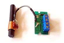
An LC circuit, also called a resonant circuit, tank circuit, or tuned circuit, is an electric circuit consisting of an inductor, represented by the letter L, and a capacitor, represented by the letter C, connected together. The circuit can act as an electrical resonator, an electrical analogue of a tuning fork, storing energy oscillating at the circuit's resonant frequency.[1]
LC circuits are used either for generating signals at a particular frequency, or picking out a signal at a particular frequency from a more complex signal; this function is called a bandpass filter. They are key components in many electronic devices, particularly radio equipment, used in circuits such as oscillators, filters, tuners and frequency mixers.[1]
An LC circuit is an idealized model since it assumes there is no dissipation of energy due to resistance. Any practical implementation of an LC circuit will always include loss resulting from small but non-zero resistance within the components and connecting wires. The purpose of an LC circuit is usually to oscillate with minimal damping, so the resistance is made as low as possible. While no practical circuit is without losses, it is nonetheless instructive to study this ideal form of the circuit to gain understanding and physical intuition. For a circuit model incorporating resistance, see RLC circuit.[1]
Terminology
The two-element LC circuit described above is the simplest type of inductor-capacitor network (or LC network). It is also referred to as a second order LC circuit to distinguish it from more complicated (higher order) LC networks with more inductors and capacitors. Such LC networks with more than two reactances may have more than one resonant frequency.
The order of the network is the order of the rational function describing the network in the complex frequency variable s. Generally, the order is equal to the number of L and C elements in the circuit and in any event cannot exceed this number.
Operation
An LC circuit, oscillating at its natural resonant frequency, can store electrical energy. See the animation at right. A capacitor stores energy in the electric field (E) between its plates, depending on the voltage across it, and an inductor stores energy in its magnetic field (B), depending on the current through it.
If an inductor is connected across a charged capacitor, current will start to flow through the inductor, building up a magnetic field around it and reducing the voltage on the capacitor. Eventually all the charge on the capacitor will be gone and the voltage across it will reach zero. However, the current will continue, because inductors oppose changes in current. The current will begin to charge the capacitor with a voltage of opposite polarity to its original charge. Due to Faraday's law, the EMF which drives the current is caused by a decrease in the magnetic field, thus the energy required to charge the capacitor is extracted from the magnetic field. When the magnetic field is completely dissipated the current will stop and the charge will again be stored in the capacitor, with the opposite polarity as before. Then the cycle will begin again, with the current flowing in the opposite direction through the inductor.
The charge flows back and forth between the plates of the capacitor, through the inductor. The energy oscillates back and forth between the capacitor and the inductor until (if not replenished from an external circuit) internal resistance makes the oscillations die out. In most applications the tuned circuit is part of a larger circuit which applies alternating current to it, driving continuous oscillations. If the frequency of the applied current is the circuit's natural resonant frequency (natural frequency below ), resonance will occur. The tuned circuit's action, known mathematically as a harmonic oscillator, is similar to a pendulum swinging back and forth, or water sloshing back and forth in a tank; for this reason the circuit is also called a tank circuit.[2] The natural frequency (that is, the frequency at which it will oscillate when isolated from any other system, as described above) is determined by the capacitance and inductance values. In typical tuned circuits in electronic equipment the oscillations are very fast, from thousands to billions of times per second.

Resonance effect
Resonance occurs when an LC circuit is driven from an external source at an angular frequency ω0 at which the inductive and capacitive reactances are equal in magnitude. The frequency at which this equality holds for the particular circuit is called the resonant frequency. The resonant frequency of the LC circuit is

where L is the inductance in henrys, and C is the capacitance in farads. The angular frequency ω0 has units of radians per second.
The equivalent frequency in units of hertz is

Applications
The resonance effect of the LC circuit has many important applications in signal processing and communications systems.
- The most common application of tank circuits is tuning radio transmitters and receivers. For example, when we tune a radio to a particular station, the LC circuits are set at resonance for that particular carrier frequency.
- A series resonant circuit provides voltage magnification.
- A parallel resonant circuit provides current magnification.
- A parallel resonant circuit can be used as load impedance in output circuits of RF amplifiers. Due to high impedance, the gain of amplifier is maximum at resonant frequency.
- Both parallel and series resonant circuits are used in induction heating.
LC circuits behave as electronic resonators, which are a key component in many applications:
Time domain solution
Kirchhoff's laws
By Kirchhoff's voltage law, the voltage across the capacitor, VC, plus the voltage across the inductor, VL must equal zero:

Likewise, by Kirchhoff's current law, the current through the capacitor equals the current through the inductor:

From the constitutive relations for the circuit elements, we also know that

Differential equation
Rearranging and substituting gives the second order differential equation

The parameter ω0, the resonant angular frequency, is defined as:

Using this can simplify the differential equation

The associated polynomial is

thus,

where j is the imaginary unit.
Solution
Thus, the complete solution to the differential equation is

and can be solved for A and B by considering the initial conditions. Since the exponential is complex, the solution represents a sinusoidal alternating current. Since the electric current I is a physical quantity, it must be real-valued. As a result, it can be shown that the constants A and B must be complex conjugates:

Now, let

Therefore,

Next, we can use Euler's formula to obtain a real sinusoid with amplitude I0, angular frequency ω0 = 1/√LC, and phase angle φ.
Thus, the resulting solution becomes:

and

Initial conditions
The initial conditions that would satisfy this result are:

and

Series LC circuit
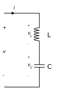
In the series configuration of the LC circuit, the inductor (L) and capacitor (C) are connected in series, as shown here. The total voltage V across the open terminals is simply the sum of the voltage across the inductor and the voltage across the capacitor. The current I into the positive terminal of the circuit is equal to the current through both the capacitor and the inductor.

Resonance
Inductive reactance magnitude XL increases as frequency increases while capacitive reactance magnitude XC decreases with the increase in frequency. At one particular frequency, these two reactances are equal in magnitude but opposite in sign; that frequency is called the resonant frequency f0 for the given circuit.
Hence, at resonance:

Solving for ω, we have

which is defined as the resonant angular frequency of the circuit. Converting angular frequency (in radians per second) into frequency (in hertz), one has

In a series configuration, XC and XL cancel each other out. In real, rather than idealised components, the current is opposed, mostly by the resistance of the coil windings. Thus, the current supplied to a series resonant circuit is a maximum at resonance.
- In the limit as f → f0 current is maximum. Circuit impedance is minimum. In this state, a circuit is called an acceptor circuit[3]
- For f < f0, XL ≪ −XC. Hence, the circuit is capacitive.
- For f > f0, XL ≫ −XC. Hence, the circuit is inductive.
Impedance
In the series configuration, resonance occurs when the complex electrical impedance of the circuit approaches zero.
First consider the impedance of the series LC circuit. The total impedance is given by the sum of the inductive and capacitive impedances:

Writing the inductive impedance as ZL = jωL and capacitive impedance as ZC = 1/jωC and substituting gives

Writing this expression under a common denominator gives

Finally, defining the natural angular frequency as

the impedance becomes

The numerator implies that in the limit as ω → ±ω0, the total impedance Z will be zero and otherwise non-zero. Therefore the series LC circuit, when connected in series with a load, will act as a band-pass filter having zero impedance at the resonant frequency of the LC circuit.
Parallel LC circuit
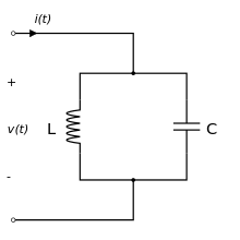
In the parallel configuration, the inductor L and capacitor C are connected in parallel, as shown here. The voltage V across the open terminals is equal to both the voltage across the inductor and the voltage across the capacitor. The total current I flowing into the positive terminal of the circuit is equal to the sum of the current flowing through the inductor and the current flowing through the capacitor:

Resonance
When XL equals XC, the reactive branch currents are equal and opposite. Hence they cancel out each other to give minimum current in the main line. Since total current is minimum, in this state the total impedance is maximum.
The resonant frequency is given by
Note that any reactive branch current is not minimum at resonance, but each is given separately by dividing source voltage (V) by reactance (Z). Hence I = V/Z, as per Ohm's law.
- At f0, the line current is minimum. The total impedance is at the maximum. In this state a circuit is called a rejector circuit.[4]
- Below f0, the circuit is inductive.
- Above f0, the circuit is capacitive.
Impedance
The same analysis may be applied to the parallel LC circuit. The total impedance is then given by:

and after substitution of ZL = jωL and ZC = 1/jωC and simplification, gives

Using
it further simplifies to

Note that

but for all other values of ω the impedance is finite. The parallel LC circuit connected in series with a load will act as band-stop filter having infinite impedance at the resonant frequency of the LC circuit. The parallel LC circuit connected in parallel with a load will act as band-pass filter.
Laplace solution
The LC circuit can be solved by Laplace transform.
Let the general equation be:


Let the differential equation of LC series be:

With initial condition:

Let define:

Gives:

Transform with Laplace:
![{\displaystyle {\mathcal {L}}\left[f(t)\right]={\mathcal {L}}\left[{\frac {\mathrm {d} ^{2}v}{\mathrm {d} t^{2}}}+\omega _{0}^{2}v\right]}](../I/m/30cbcf2f1819cc4f603a0a2ad3a45811b97fc4e4.svg)


Then antitransform:
![{\displaystyle v(t)=v_{0}\cos(\omega _{0}t)+{\frac {v'_{0}}{\omega _{0}}}\sin(\omega _{0}t)+{\mathcal {L}}^{-1}\left[{\frac {F(s)}{s^{2}+\omega _{0}^{2}}}\right]}](../I/m/45c285c8ecf64f776538ac642c546731c90298f4.svg)
In case input voltage is Heaviside step function:

![{\displaystyle {\mathcal {L}}^{-1}\left[\omega _{0}^{2}{\frac {V_{in}(s)}{s^{2}+\omega _{0}^{2}}}\right]={\mathcal {L}}^{-1}\left[\omega _{0}^{2}M{\frac {1}{s(s^{2}+\omega _{0}^{2})}}\right]=M(1-\cos(\omega _{0}t))}](../I/m/ef60af8194e4e7c94c43a8f36e04b4f0899d889f.svg)

In case input voltage is sinusoidal function:

![{\displaystyle {\mathcal {L}}^{-1}\left[\omega _{0}^{2}{\frac {1}{s^{2}+\omega _{0}^{2}}}{\frac {U\omega _{f}}{s^{2}+\omega _{f}^{2}}}\right]={\mathcal {L}}^{-1}\left[{\frac {\omega _{0}^{2}U\omega _{f}}{\omega _{f}^{2}-\omega _{0}^{2}}}\left({\frac {1}{s^{2}+\omega _{0}^{2}}}-{\frac {1}{s^{2}+\omega _{f}^{2}}}\right)\right]={\frac {\omega _{0}^{2}U\omega _{f}}{\omega _{f}^{2}-\omega _{0}^{2}}}\left({\frac {1}{\omega _{0}}}\sin(\omega _{0}t)-{\frac {1}{\omega _{f}}}\sin(\omega _{f}t)\right)}](../I/m/dd8a9fa8b4b72855ce52a23d207d1e1891ed54cb.svg)

History
The first evidence that a capacitor and inductor could produce electrical oscillations was discovered in 1826 by French scientist Felix Savary.[5][6] He found that when a Leyden jar was discharged through a wire wound around an iron needle, sometimes the needle was left magnetized in one direction and sometimes in the opposite direction. He correctly deduced that this was caused by a damped oscillating discharge current in the wire, which reversed the magnetization of the needle back and forth until it was too small to have an effect, leaving the needle magnetized in a random direction. American physicist Joseph Henry repeated Savary's experiment in 1842 and came to the same conclusion, apparently independently.[7][8] British scientist William Thomson (Lord Kelvin) in 1853 showed mathematically that the discharge of a Leyden jar through an inductance should be oscillatory, and derived its resonant frequency.[5][7][8] British radio researcher Oliver Lodge, by discharging a large battery of Leyden jars through a long wire, created a tuned circuit with its resonant frequency in the audio range, which produced a musical tone from the spark when it was discharged.[7] In 1857, German physicist Berend Wilhelm Feddersen photographed the spark produced by a resonant Leyden jar circuit in a rotating mirror, providing visible evidence of the oscillations.[5][7][8] In 1868, Scottish physicist James Clerk Maxwell calculated the effect of applying an alternating current to a circuit with inductance and capacitance, showing that the response is maximum at the resonant frequency.[5] The first example of an electrical resonance curve was published in 1887 by German physicist Heinrich Hertz in his pioneering paper on the discovery of radio waves, showing the length of spark obtainable from his spark-gap LC resonator detectors as a function of frequency.[5]
One of the first demonstrations of resonance between tuned circuits was Lodge's "syntonic jars" experiment around 1889.[5][7] He placed two resonant circuits next to each other, each consisting of a Leyden jar connected to an adjustable one-turn coil with a spark gap. When a high voltage from an induction coil was applied to one tuned circuit, creating sparks and thus oscillating currents, sparks were excited in the other tuned circuit only when the circuits were adjusted to resonance. Lodge and some English scientists preferred the term "syntony" for this effect, but the term "resonance" eventually stuck.[5] The first practical use for LC circuits was in the 1890s in spark-gap radio transmitters to allow the receiver and transmitter to be tuned to the same frequency. The first patent for a radio system that allowed tuning was filed by Lodge in 1897, although the first practical systems were invented in 1900 by Italian radio pioneer Guglielmo Marconi.[5]
See also
References
- 1 2 3 Reviews, C. T. I. (2016-09-26). Electricity and Magnetism. Cram101 Textbook Reviews. ISBN 9781467279659.
- ↑ Rao, B. Visvesvara; et al. (2012). Electronic Circuit Analysis. India: Pearson Education India. p. 13.6. ISBN 9332511748.
- ↑ What is Acceptor Circuit
- ↑ "rejector circuit | Definition of rejector circuit in English by Oxford Dictionaries". Oxford Dictionaries | English. Retrieved 2018-09-20.
- 1 2 3 4 5 6 7 8 Blanchard, Julian (October 1941). "The History of Electrical Resonance". Bell System Technical Journal. U.S.: American Telephone & Telegraph Co. 20 (4): 415. doi:10.1002/j.1538-7305.1941.tb03608.x. Retrieved 2011-03-29.
- ↑ Savary, Felix (1827). "Memoirs sur l'Aimentation". Annales de Chimie et de Physique. Paris: Masson. 34: 5–37.
- 1 2 3 4 5 Kimball, Arthur Lalanne (1917). A College Text-book of Physics (2nd ed.). New York: Henry Hold. pp. 516–517.
- 1 2 3 Huurdeman, Anton A. (2003). The Worldwide History of Telecommunications. U.S.: Wiley-IEEE. pp. 199–200. ISBN 0-471-20505-2.
External links
| The Wikibook Circuit Idea has a page on the topic of: How do We Create Sinusoidal Oscillations? |
- An electric pendulum by Tony Kuphaldt is a classical story about the operation of LC tank
- How the parallel-LC circuit stores energy is another excellent LC resource.