Spinodal
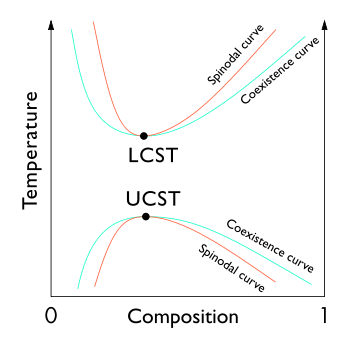
In thermodynamics, the limit of local stability with respect to small fluctuations is clearly defined by the condition that the second derivative of Gibbs free energy is zero. The locus of these points (the inflection point within a G-x or G-c curve, Gibbs free energy as a function of composition) is known as the spinodal curve.[1][2][3] For compositions within this curve, infinitesimally small fluctuations in composition and density will lead to phase separation via spinodal decomposition. Outside of the curve, the solution will be at least metastable with respect to fluctuations.[3] In other words, outside the spinodal curve some careful process may obtain a single phase system.[3] Inside it, only processes far from thermodynamic equilibrium, such as physical vapor deposition, will enable one to prepare single phase compositions.[4] The local points of coexisting compositions, defined by the common tangent construction, are known as binodal (coexistence) curve, which denotes the minimum-energy equilibrium state of the system. Increasing temperature results in a decreasing difference between mixing entropy and mixing enthalpy, thus, the coexisting compositions come closer. The binodal curve forms the bases for the miscibility gap in a phase diagram. Since the free energy of mixture changes with temperature and concentration, the binodal and spinodal meet at the critical or consulate temperature and composition.[5]
Criterion
For binary solutions, the thermodynamic criterion which defines the spinodal curve is that the second derivative of free energy with respect to density or some composition variable is zero.[3][6][7]
Critical point
Extrema of the spinodal in temperature with respect to the composition variable coincide with ones of the binodal curve and are known as critical points.[7]
Isothermal liquid-liquid equilibria
In the case of ternary isothermal liquid-liquid equilibria, the spinodal curve (obtained from the Hessian matrix) and the corresponding critical point can be used to help the experimental data correlation process.[8][9][10]
References
- ↑ G. Astarita: Thermodynamics: An Advanced Textbook for Chemical Engineers (Springer 1990), chaps 4, 8, 9, 12.
- ↑ Sandler S. I., Chemical and Engineering Thermodynamics. 1999 John Wiley & Sons, Inc., p 571.
- 1 2 3 4 Koningsveld K., Stockmayer W. H., Nies, E., Polymer Phase Diagrams: A Textbook. 2001 Oxford, p 12.
- ↑ P.H. Mayrhofer et al. Progress in Materials Science 51 (2006) 1032-1114 doi:10.1016/j.pmatsci.2006.02.002
- ↑ Cahn RW, Haasen P. Physical metallurgy. 4th ed. Cambridge: Univ Press; 1996
- ↑ Sandler S. I., Chemical and Engineering Thermodynamics. 1999 John Wiley & Sons, Inc., p 557.
- 1 2 Koningsveld K., Stockmayer W. H., Nies, E., Polymer Phase Diagrams: A Textbook. 2001 Oxford, pp 46-47.
- ↑ Marcilla, A.; Serrano, M.D.; Reyes-Labarta, J.A.; Olaya, M.M. (2012). "Checking Liquid-Liquid Critical Point Conditions and their Application in Ternary Systems". Industrial & Engineering Chemistry Research. 51 (13): 5098-5102. doi:10.1021/ie202793r.
- ↑ Marcilla, A.; Reyes-Labarta, J.A.; Serrano, M.D.; Olaya, M.M. (2011). "GE Models and Algorithms for Condensed Phase Equilibrium Data Regression in Ternary Systems: Limitations and Proposals". The Open Thermodynamics Journal. 5: 48-62. doi:10.2174/1874396X01105010048.
- ↑ Graphical User Interface, (GUI). "Topological Analysis of the Gibbs Energy Function (Liquid-Liquid Equilibrium Correlation Data. Including a Thermodinamic Review and Tie-lines/Hessian matrix analysis)". Institutional Repository (RUA). University of Alicante (Reyes-Labarta et al. 2015-18).
| State |  | |
|---|---|---|
| Low energy | ||
| High energy | ||
| Other states | ||
| Transitions |
| |
| Quantities | ||
| Concepts | ||