Spatial heterogeneity
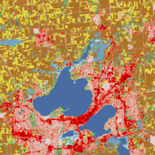
Spatial heterogeneity is a property generally ascribed to a landscape or to a population. It refers to the uneven distribution of various concentrations of each species within an area. A landscape with spatial heterogeneity has a mix of concentrations of multiple species of plants or animals (biological), or of terrain formations (geological), or environmental characteristics (e.g. rainfall, temperature, wind) filling its area. A population showing spatial heterogeneity is one where various concentrations of individuals of this species are unevenly distributed across an area; nearly synonymous with "patchily distributed."
Environments with a wide variety of habitats such as different topographies, soil types, and climates are able to accommodate a greater amount of species. The leading scientific explanation for this is that when organisms can finely subdivide a landscape into unique suitable habitats, more species can coexist in a landscape without competition, a phenomenon termed "niche partitioning." Spatial heterogeneity is a concept parallel to ecosystem productivity, the species richness of animals is directly related to the species richness of plants in a certain habitat. Vegetation serves as food sources, habitats, and so on. Therefore, if vegetation is scarce, the animal populations will be as well. The more plant species there are in an ecosystem, the greater variety of microhabitats there are. Plant species richness directly reflects spatial heterogeneity in an ecosystem.
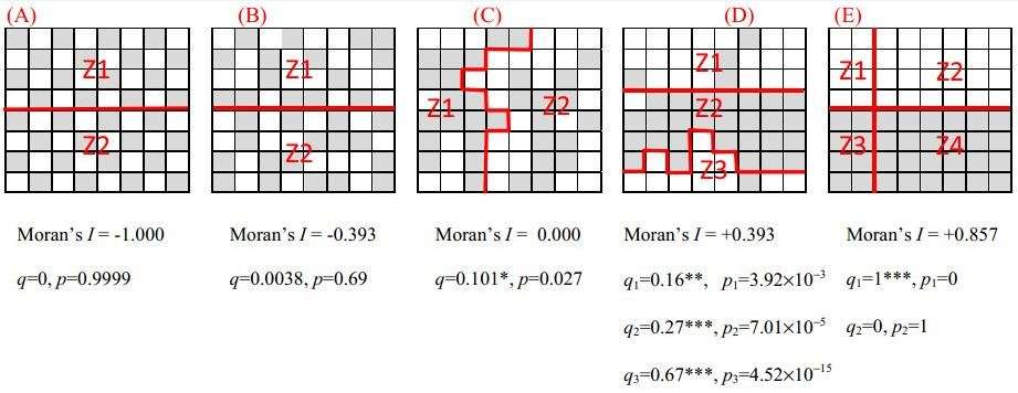
Spatial heterogeneity could be either local or stratified, the former is called spatial local heterogeneity, referring to the phenomena that the value of an attribute at one site is different from its surrounding, such as hotspot or cold spot; the latter is called spatial stratified heterogeneity, referring to the phenomena that the within strata variance is less than the between strata variance, such as ecological zones and landuse classes. Spatial local heterogeneity can be tested by LISA, Gi and SatScan, while spatial stratified heterogeneity of an attribute can be measured by geographical detector q-statistic:[1]

where a population is partitioned into h = 1, ..., L strata; N stands for the size of the population, σ2 stands for variance of the attribute. The value of q is within [0, 1], 0 indicates no spatial stratified heterogeneity, 1 indicates perfect spatial stratified heterogeneity.The value of q indicates the percent of the variance of an attribute explained by the stratification.The q follows a noncentral F probability density function.
Spatial heterogeneity can be re-phrased as scaling hierarchy of far more small things than large ones. It has been formulated as a scaling law.
[2]
Spatial heterogeneity or scaling hierarchy can be measured or quantified by ht-index - a head/tail breaks induced number. [3] [4]
See also
References
- ↑ Wang JF, Zhang TL, Fu BJ. 2016. A measure of spatial stratified heterogeneity. Ecological Indicators 67: 250-256.
- ↑ Jiang B. 2015. Geospatial analysis requires a different way of thinking: The problem of spatial heterogeneity. GeoJournal 80(1), 1-13.
- ↑ Jiang B. and Yin J. 2014. Ht-index for quantifying the fractal or scaling structure of geographic features, Annals of the Association of American Geographers, 104(3), 530–541.
- ↑ Jiang B. 2013. Head/tail breaks: A new classification scheme for data with a heavy-tailed distribution, The Professional Geographer, 65 (3), 482 – 494.