Rayleigh–Taylor instability

RT instability fingers evident in the Crab Nebula

The Rayleigh–Taylor instability, or RT instability (after Lord Rayleigh and G. I. Taylor), is an instability of an interface between two fluids of different densities which occurs when the lighter fluid is pushing the heavier fluid.^[1]^[2]^[3] Examples include the behavior of water suspended above oil in the gravity of Earth,^[2] mushroom clouds like those from volcanic eruptions and atmospheric nuclear explosions,^[4] supernova explosions in which expanding core gas is accelerated into denser shell gas,^[5]^[6] instabilities in plasma fusion reactors and ^[7] inertial confinement fusion.^[8]

Water suspended atop oil is an everyday example of Rayleigh–Taylor instability, and it may be modeled by two completely plane-parallel layers of immiscible fluid, the more dense on top of the less dense one and both subject to the Earth's gravity. The equilibrium here is unstable to any perturbations or disturbances of the interface: if a parcel of heavier fluid is displaced downward with an equal volume of lighter fluid displaced upwards, the potential energy of the configuration is lower than the initial state. Thus the disturbance will grow and lead to a further release of potential energy, as the more dense material moves down under the (effective) gravitational field, and the less dense material is further displaced upwards. This was the set-up as studied by Lord Rayleigh.^[2] The important insight by G. I. Taylor was his realisation that this situation is equivalent to the situation when the fluids are accelerated, with the less dense fluid accelerating into the more dense fluid.^[2] This occurs deep underwater on the surface of an expanding bubble and in a nuclear explosion.^[9]

As the RT instability develops, the initial perturbations progress from a linear growth phase into a non-linear growth phase, eventually developing "plumes" flowing upwards (in the gravitational buoyancy sense) and "spikes" falling downwards. In the linear phase, equations can be linearized and the amplitude of perturbations is growing exponentially with time. In the non-linear phase, perturbation amplitude is too large for the non-linear terms to be neglected. In general, the density disparity between the fluids determines the structure of the subsequent non-linear RT instability flows (assuming other variables such as surface tension and viscosity are negligible here). The difference in the fluid densities divided by their sum is defined as the Atwood number, A. For A close to 0, RT instability flows take the form of symmetric "fingers" of fluid; for A close to 1, the much lighter fluid "below" the heavier fluid takes the form of larger bubble-like plumes.^[1]

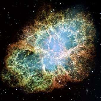
This process is evident not only in many terrestrial examples, from salt domes to weather inversions, but also in astrophysics and electrohydrodynamics. RT instability structure is also evident in the Crab Nebula, in which the expanding pulsar wind nebula powered by the Crab pulsar is sweeping up ejected material from the supernova explosion 1000 years ago.^[10] The RT instability has also recently been discovered in the Sun's outer atmosphere, or solar corona, when a relatively dense solar prominence overlies a less dense plasma bubble.^[11] This latter case is an clear example of the magnetically modulated RT instability.^[12]^[13]

Note that the RT instability is not to be confused with the Plateau–Rayleigh instability (also known as Rayleigh instability) of a liquid jet. This instability, sometimes called the hosepipe (or firehose) instability, occurs due to surface tension, which acts to break a cylindrical jet into a stream of droplets having the same total volume but higher surface area.

Many people have witnessed the RT instability by looking at a lava lamp, although some might claim this is more accurately described as an example of Rayleigh–Bénard convection due to the active heating of the fluid layer at the bottom of the lamp.

Linear stability analysis

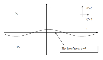
Base state of the Rayleigh–Taylor instability. Gravity points downwards.

The inviscid two-dimensional Rayleigh–Taylor (RT) instability provides an excellent springboard into the mathematical study of stability because of the simple nature of the base state.^[14] This is the equilibrium state that exists before any perturbation is added to the system, and is described by the mean velocity field $U(x,z)=W(x,z)=0,\,$ where the gravitational field is ${\textbf {g}}=-g{\hat {{\textbf {z}}}}.\,$ An interface at $z=0\,$ separates the fluids of densities $\rho _{G}\,$ in the upper region, and $\rho _{L}\,$ in the lower region. In this section it is shown that when the heavy fluid sits on top, the growth of a small perturbation at the interface is exponential, and takes place at the rate^[2]

\exp(\gamma \,t)\;,\qquad {\text{with}}\quad \gamma ={{\sqrt {{\mathcal {A}}g\alpha }}}\quad {\text{and}}\quad {\mathcal {A}}={\frac {\rho _{{{\text{heavy}}}}-\rho _{{{\text{light}}}}}{\rho _{{{\text{heavy}}}}+\rho _{{{\text{light}}}}}},\,

where $\gamma \,$ is the temporal growth rate, $\alpha \,$ is the spatial wavenumber and ${\mathcal {A}}\,$ is the Atwood number.

Details of the linear stability analysis^[14] A similar derivation appears in,^[12] §92, pp. 433–435.

The perturbation introduced to the system is described by a velocity field of infinitesimally small amplitude, $(u'(x,z,t),w'(x,z,t)).\,$ Because the fluid is assumed incompressible, this velocity field has the streamfunction representation

{\textbf {u}}'=(u'(x,z,t),w'(x,z,t))=(\psi _{z},-\psi _{x}),\,

where the subscripts indicate partial derivatives. Moreover, in an initially stationary incompressible fluid, there is no vorticity, and the fluid stays irrotational, hence $\nabla \times {\textbf {u}}'=0\,$ . In the streamfunction representation, $\nabla ^{2}\psi =0.\,$ Next, because of the translational invariance of the system in the x-direction, it is possible to make the ansatz

\psi \left(x,z,t\right)=e^{{i\alpha \left(x-ct\right)}}\Psi \left(z\right),\,

where $\alpha \,$ is a spatial wavenumber. Thus, the problem reduces to solving the equation

\left(D^{2}-\alpha ^{2}\right)\Psi _{j}=0,\,\,\,\ D={\frac {d}{dz}},\,\,\,\ j=L,G.\,

The domain of the problem is the following: the fluid with label 'L' lives in the region $-\infty <z\leq 0\,$ , while the fluid with the label 'G' lives in the upper half-plane $0\leq z<\infty \,$ . To specify the solution fully, it is necessary to fix conditions at the boundaries and interface. This determines the wave speed c, which in turn determines the stability properties of the system.

The first of these conditions is provided by details at the boundary. The perturbation velocities $w'_{i}\,$ should satisfy a no-flux condition, so that fluid does not leak out at the boundaries $z=\pm \infty .\,$ Thus, $w_{L}'=0\,$ on $z=-\infty \,$ , and $w_{G}'=0\,$ on $z=\infty \,$ . In terms of the streamfunction, this is

\Psi _{L}\left(-\infty \right)=0,\qquad \Psi _{G}\left(\infty \right)=0.\,

The other three conditions are provided by details at the interface $z=\eta \left(x,t\right)\,$ .

Continuity of vertical velocity: At $z=\eta$ , the vertical velocities match, $w'_{L}=w'_{G}\,$ . Using the streamfunction representation, this gives

\Psi _{L}\left(\eta \right)=\Psi _{G}\left(\eta \right).\,

Expanding about $z=0\,$ gives

\Psi _{L}\left(0\right)=\Psi _{G}\left(0\right)+{\text{H.O.T.}},\,

where H.O.T. means 'higher-order terms'. This equation is the required interfacial condition.

The free-surface condition: At the free surface $z=\eta \left(x,t\right)\,$ , the kinematic condition holds:

{\frac {\partial \eta }{\partial t}}+u'{\frac {\partial \eta }{\partial x}}=w'\left(\eta \right).\,

Linearizing, this is simply

{\frac {\partial \eta }{\partial t}}=w'\left(0\right),\,

where the velocity $w'\left(\eta \right)\,$ is linearized on to the surface $z=0\,$ . Using the normal-mode and streamfunction representations, this condition is $c\eta =\Psi \,$ , the second interfacial condition.

Pressure relation across the interface: For the case with surface tension, the pressure difference over the interface at $z=\eta$ is given by the Young–Laplace equation:

p_{G}\left(z=\eta \right)-p_{L}\left(z=\eta \right)=\sigma \kappa ,\,

where σ is the surface tension and κ is the curvature of the interface, which in a linear approximation is

\kappa =\nabla ^{2}\eta =\eta _{xx}.\,

Thus,

p_{G}\left(z=\eta \right)-p_{L}\left(z=\eta \right)=\sigma \eta _{{xx}}.\,

However, this condition refers to the total pressure (base+perturbed), thus

\left[P_{G}\left(\eta \right)+p'_{G}\left(0\right)\right]-\left[P_{L}\left(\eta \right)+p'_{L}\left(0\right)\right]=\sigma \eta _{{xx}}.\,

(As usual, The perturbed quantities can be linearized onto the surface z=0.) Using hydrostatic balance, in the form

P_{L}=-\rho _{L}gz+p_{0},\qquad P_{G}=-\rho _{G}gz+p_{0},\,

this becomes

p'_{G}-p'_{L}=g\eta \left(\rho _{G}-\rho _{L}\right)+\sigma \eta _{{xx}},\qquad {\text{on }}z=0.\,

The perturbed pressures are evaluated in terms of streamfunctions, using the horizontal momentum equation of the linearised Euler equations for the perturbations,

{\frac {\partial u_{i}'}{\partial t}}=-{\frac {1}{\rho _{i}}}{\frac {\partial p_{i}'}{\partial x}}\,

with

i=L,G,\,

to yield

p_{i}'=\rho _{i}cD\Psi _{i},\qquad i=L,G.\,

Putting this last equation and the jump condition on $p'_{G}-p'_{L}$ together,

c\left(\rho _{G}D\Psi _{G}-\rho _{L}D\Psi _{L}\right)=g\eta \left(\rho _{G}-\rho _{L}\right)+\sigma \eta _{{xx}}.\,

Substituting the second interfacial condition $c\eta =\Psi \,$ and using the normal-mode representation, this relation becomes

c^{2}\left(\rho _{G}D\Psi _{G}-\rho _{L}D\Psi _{L}\right)=g\Psi \left(\rho _{G}-\rho _{L}\right)-\sigma \alpha ^{2}\Psi ,\,

where there is no need to label $\Psi \,$ (only its derivatives) because $\Psi _{L}=\Psi _{G}\,$ at $z=0.\,$

Solution

Now that the model of stratified flow has been set up, the solution is at hand. The streamfunction equation $\left(D^{2}-\alpha ^{2}\right)\Psi _{i}=0,\,$ with the boundary conditions $\Psi \left(\pm \infty \right)\,$ has the solution

\Psi _{L}=A_{L}e^{{\alpha z}},\qquad \Psi _{G}=A_{G}e^{{-\alpha z}}.\,

The first interfacial condition states that $\Psi _{L}=\Psi _{G}\,$ at $z=0\,$ , which forces $A_{L}=A_{G}=A.\,$ The third interfacial condition states that

c^{2}\left(\rho _{G}D\Psi _{G}-\rho _{L}D\Psi _{L}\right)=g\Psi \left(\rho _{G}-\rho _{L}\right)-\sigma \alpha ^{2}\Psi .\,

Plugging the solution into this equation gives the relation

Ac^{2}\alpha \left(-\rho _{G}-\rho _{L}\right)=Ag\left(\rho _{G}-\rho _{L}\right)-\sigma \alpha ^{2}A.\,

The A cancels from both sides and we are left with

c^{2}={\frac {g}{\alpha }}{\frac {\rho _{L}-\rho _{G}}{\rho _{L}+\rho _{G}}}+{\frac {\sigma \alpha }{\rho _{L}+\rho _{G}}}.\,

To understand the implications of this result in full, it is helpful to consider the case of zero surface tension. Then,

c^{2}={\frac {g}{\alpha }}{\frac {\rho _{L}-\rho _{G}}{\rho _{L}+\rho _{G}}},\qquad \sigma =0,\,

and clearly

If $\rho _{G}<\rho _{L}\,$ , $c^{2}>0\,$ and c is real. This happens when the

lighter fluid sits on top;

If $\rho _{G}>\rho _{L}\,$ , $c^{2}<0\,$ and c is purely imaginary. This happens

when the heavier fluid sits on top.

Now, when the heavier fluid sits on top, $c^{2}<0\,$ , and

c=\pm i{\sqrt {{\frac {g{\mathcal {A}}}{\alpha }}}},\qquad {\mathcal {A}}={\frac {\rho _{G}-\rho _{L}}{\rho _{G}+\rho _{L}}},\,

where ${\mathcal {A}}\,$ is the Atwood number. By taking the positive solution, we see that the solution has the form

\Psi \left(x,z,t\right)=Ae^{{-\alpha |z|}}\exp \left[i\alpha \left(x-ct\right)\right]=A\exp \left(\alpha {\sqrt {{\frac {g{\tilde {{\mathcal {A}}}}}{\alpha }}}}t\right)\exp \left(i\alpha x-\alpha |z|\right)\,

and this is associated to the interface position η by: $c\eta =\Psi .\,$ Now define $B=A/c.\,$

The time evolution of the free interface elevation $z=\eta (x,t),\,$ initially at $\eta (x,0)=\Re \left\{B\,\exp \left(i\alpha x\right)\right\},\,$ is given by:

\eta =\Re \left\{B\,\exp \left({\sqrt {{\mathcal {A}}g\alpha }}\,t\right)\exp \left(i\alpha x\right)\right\}\,

which grows exponentially in time. Here B is the amplitude of the initial perturbation, and $\Re \left\{\cdot \right\}\,$ denotes the real part of the complex valued expression between brackets.

In general, the condition for linear instability is that the imaginary part of the "wave speed" c is positive. Finally, restoring the surface tension makes c² less negative and is therefore stabilizing. Indeed, there is a range of short waves for which the surface tension stabilizes the system and prevents the instability forming.

Vorticity explanation

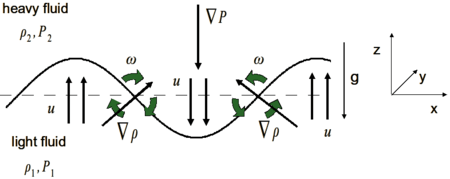
Visualization of an unstable Rayleigh–Taylor instability configuration where baroclinic torque at the interface creates vorticity and induces a velocity field that increases the baroclinic torque. Here ω is vorticity, p is pressure, ρ is density, u is velocity and g is gravity. The thick circular arrows represent the velocity field created by the vortex.

The RT instability can be seen as the result of baroclinic torque created by the misalignment of the pressure and density gradients at the perturbed interface, as described by the two-dimensional inviscid vorticity equation, ${\frac {D\omega }{Dt}}={\frac {1}{\rho ^{2}}}\nabla \rho \times \nabla p$ , where ω is vorticity, ρ density and p is the pressure. In this case the dominant pressure gradient is hydrostatic, resulting from the acceleration.

When in the unstable configuration, for a particular harmonic component of the initial perturbation, the torque on the interface creates vorticity that will tend to increase the misalignment of the gradient vectors. This in turn creates additional vorticity, leading to further misalignment. This concept is depicted in the figure, where it is observed that the two counter-rotating vortices have velocity fields that sum at the peak and trough of the perturbed interface. In the stable configuration, the vorticity, and thus the induced velocity field, will be in a direction that decreases the misalignment and therefore stabilizes the system.^[15]^[16]

Late-time behaviour

Hydrodynamics simulation of a single "finger" of the Rayleigh–Taylor instability^[17] Note the formation of Kelvin–Helmholtz instabilities, in the second and later snapshots shown (starting initially around the level

y=0

), as well as the formation of a "mushroom cap" at a later stage in the third and fourth frame in the sequence.

The analysis in the previous section breaks down when the amplitude of the perturbation is large. The growth then becomes non-linear as the spikes and bubbles of the instability tangle and roll up into vortices. Then, as in the figure, numerical simulation of the full problem is required to describe the system.

Stages of development and eventual evolution into turbulent mixing

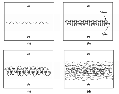
This figure represents the evolution of the Rayleigh–Taylor instability from small wavelength perturbations at the interface (a) which grow into the ubiquitous mushroom shaped spikes (fluid structures of heavy into light fluid) and bubbles (fluid structures of light into heavy fluid) (b) and these fluid structures interact due to bubble merging and competition (c) eventually developing into a mixing region (d). Here ρ2 represents the heavy fluid and ρ1 represents the light fluid. Gravity is acting downward and the system is RT unstable.

The evolution of the RTI follows four main stages.^[1] In the first stage, the perturbation amplitudes are small when compared to their wavelengths, the equations of motion can be linearized, resulting in exponential instability growth. In the early portion of this stage, a sinusoidal initial perturbation retains its sinusoidal shape. However, after the end of this first stage, when non-linear effects begin to appear, one observes the beginnings of the formation of the ubiquitous mushroom-shaped spikes (fluid structures of heavy fluid growing into light fluid) and bubbles (fluid structures of light fluid growing into heavy fluid). The growth of the mushroom structures continues in the second stage and can be modeled using buoyancy drag models, resulting in a growth rate that is approximately constant in time. At this point, nonlinear terms in the equations of motion can no longer be ignored. The spikes and bubbles then begin to interact with one another in the third stage. Bubble merging takes place, where the nonlinear interaction of mode coupling acts to combine smaller spikes and bubbles to produce larger ones. Also, bubble competition takes places, where spikes and bubbles of smaller wavelength that have become saturated are enveloped by larger ones that have not yet saturated. This eventually develops into a region of turbulent mixing,which is the fourth and final stage in the evolution. It is generally assumed that the mixing region that finally develops is self-similar and turbulent, provided that the Reynolds number is sufficiently large.^[15]

Notes

1 2 3 Sharp, D.H. (1984). "An Overview of Rayleigh-Taylor Instability" (Submitted manuscript). Physica D. 12 (1): 3–18. Bibcode:1984PhyD...12....3S. doi:10.1016/0167-2789(84)90510-4.
1 2 3 4 5 Drazin (2002) pp. 50–51.
↑ David Youngs (ed.). "Rayleigh–Taylor instability and mixing". Scholarpedia.
↑ https://gizmodo.com/why-nuclear-bombs-create-mushroom-clouds-1468107869
↑ Wang, C.-Y. & Chevalier R. A. (2000). "Instabilities and Clumping in Type Ia Supernova Remnants". The Astrophysical Journal. 549 (2): 1119–1134. arXiv:astro-ph/0005105v1. Bibcode:2001ApJ...549.1119W. doi:10.1086/319439.
↑ Hillebrandt, W.; Höflich, P. (1992). "Supernova 1987a in the Large Magellanic Cloud". In R. J. Tayler. Stellar Astrophysics. CRC Press. pp. 249–302. ISBN 978-0-7503-0200-5. . See page 274.
↑ Chen, H. B.; Hilko, B.; Panarella, E. (1994). "The Rayleigh–Taylor instability in the spherical pinch". Journal of Fusion Energy. 13 (4): 275–280. Bibcode:1994JFuE...13..275C. doi:10.1007/BF02215847.
↑ Betti, R.; Goncharov, V.N.; McCrory, R.L.; Verdon, C.P. (1998). "Growth rates of the ablative Rayleigh–Taylor instability in inertial confinement fusion". Physics of Plasmas. 5 (5): 1446–1454. Bibcode:1998PhPl....5.1446B. doi:10.1063/1.872802.
↑ John Pritchett (1971). "EVALUATION OF VARIOUS THEORETICAL MODELS FOR UNDERWATER EXPLOSION" (PDF). U.S. Government. p. 86. Retrieved October 9, 2012.
↑ Hester, J. Jeff (2008). "The Crab Nebula: an Astrophysical Chimera". Annual Review of Astronomy and Astrophysics. 46: 127–155. Bibcode:2008ARA&A..46..127H. doi:10.1146/annurev.astro.45.051806.110608.
↑ Berger, Thomas E.; Slater, Gregory; Hurlburt, Neal; Shine, Richard; et al. (2010). "Quiescent Prominence Dynamics Observed with the Hinode Solar Optical Telescope. I. Turbulent Upflow Plumes". The Astrophysical Journal. 716 (2): 1288–1307. Bibcode:2010ApJ...716.1288B. doi:10.1088/0004-637X/716/2/1288.
1 2 Chandrasekhar, S. (1981). Hydrodynamic and Hydromagnetic Stability. Dover. ISBN 978-0-486-64071-6. . See Chap. X.
↑ Hillier, A.; Berger, Thomas; Isobe, Hiroaki; Shibata, Kazunari (2012). "Numerical Simulations of the Magnetic Rayleigh-Taylor Instability in the Kippenhahn-Schl{\"u}ter Prominence Model. I. Formation of Upflows". The Astrophysical Journal. 716 (2): 120–133. Bibcode:2012ApJ...746..120H. doi:10.1088/0004-637X/746/2/120.
1 2 Drazin (2002) pp. 48–52.
1 2 Roberts, M.S.; Jacobs, J.W. (2015). "The effects of forced small-wavelength,finite-bandwidth initial perturbations and miscibility on the turbulent Rayleigh Taylor instability". Journal of Fluid Mechanics. 787: 50–83. Bibcode:2016JFM...787...50R. doi:10.1017/jfm.2015.599.
↑ Roberts, M.S. (2012). "Experiments and Simulations on the Incompressible, Rayleigh-Taylor Instability with Small Wavelength Initial Perturbations". University of Arizona Dissertations.
↑ Li, Shengtai & Hui Li. "Parallel AMR Code for Compressible MHD or HD Equations". Los Alamos National Laboratory. Retrieved 2006-09-05.

References

Original research papers

Rayleigh, Lord (John William Strutt) (1883). "Investigation of the character of the equilibrium of an incompressible heavy fluid of variable density". Proceedings of the London Mathematical Society. 14: 170–177. doi:10.1112/plms/s1-14.1.170. (Original paper is available at: https://www.irphe.fr/~clanet/otherpaperfile/articles/Rayleigh/rayleigh1883.pdf .)
Taylor, Sir Geoffrey Ingram (1950). "The instability of liquid surfaces when accelerated in a direction perpendicular to their planes". Proceedings of the Royal Society of London. Series A, Mathematical and Physical Sciences. 201 (1065): 192–196. Bibcode:1950RSPSA.201..192T. doi:10.1098/rspa.1950.0052.

Other

Chandrasekhar, Subrahmanyan (1981). Hydrodynamic and Hydromagnetic Stability. Dover Publications. ISBN 978-0-486-64071-6.
Drazin, P. G. (2002). Introduction to hydrodynamic stability. Cambridge University Press. ISBN 978-0-521-00965-2. xvii+238 pages.
Drazin, P. G.; Reid, W. H. (2004). Hydrodynamic stability (2nd ed.). Cambridge: Cambridge University Press. ISBN 978-0-521-52541-1. 626 pages.

External links

This article is issued from Wikipedia. The text is licensed under Creative Commons - Attribution - Sharealike. Additional terms may apply for the media files.

[Sharp84-1] 1 2 3 Sharp, D.H. (1984). "An Overview of Rayleigh-Taylor Instability" (Submitted manuscript). Physica D. 12 (1): 3–18. Bibcode:1984PhyD...12....3S. doi:10.1016/0167-2789(84)90510-4.

[Drazin_50_51-2] 1 2 3 4 5 Drazin (2002) pp. 50–51.

[3] David Youngs (ed.). "Rayleigh–Taylor instability and mixing". Scholarpedia.

[4] ttps://gizmodo.com/why-nuclear-bombs-create-mushroom-clouds-1468107869

[5] Wang, C.-Y. & Chevalier R. A. (2000). "Instabilities and Clumping in Type Ia Supernova Remnants". The Astrophysical Journal. 549 (2): 1119–1134. arXiv:astro-ph/0005105v1. Bibcode:2001ApJ...549.1119W. doi:10.1086/319439.

[6] Hillebrandt, W.; Höflich, P. (1992). "Supernova 1987a in the Large Magellanic Cloud". In R. J. Tayler. Stellar Astrophysics. CRC Press. pp. 249–302. ISBN 978-0-7503-0200-5. . See page 274.

[7] Chen, H. B.; Hilko, B.; Panarella, E. (1994). "The Rayleigh–Taylor instability in the spherical pinch". Journal of Fusion Energy. 13 (4): 275–280. Bibcode:1994JFuE...13..275C. doi:10.1007/BF02215847.

[8] Betti, R.; Goncharov, V.N.; McCrory, R.L.; Verdon, C.P. (1998). "Growth rates of the ablative Rayleigh–Taylor instability in inertial confinement fusion". Physics of Plasmas. 5 (5): 1446–1454. Bibcode:1998PhPl....5.1446B. doi:10.1063/1.872802.

[9] John Pritchett (1971). "EVALUATION OF VARIOUS THEORETICAL MODELS FOR UNDERWATER EXPLOSION" (PDF). U.S. Government. p. 86. Retrieved October 9, 2012.

[Hester2008-10] Hester, J. Jeff (2008). "The Crab Nebula: an Astrophysical Chimera". Annual Review of Astronomy and Astrophysics. 46: 127–155. Bibcode:2008ARA&A..46..127H. doi:10.1146/annurev.astro.45.051806.110608.

[Berger_2010-11] Berger, Thomas E.; Slater, Gregory; Hurlburt, Neal; Shine, Richard; et al. (2010). "Quiescent Prominence Dynamics Observed with the Hinode Solar Optical Telescope. I. Turbulent Upflow Plumes". The Astrophysical Journal. 716 (2): 1288–1307. Bibcode:2010ApJ...716.1288B. doi:10.1088/0004-637X/716/2/1288.

[Chandra_81-12] 1 2 Chandrasekhar, S. (1981). Hydrodynamic and Hydromagnetic Stability. Dover. ISBN 978-0-486-64071-6. . See Chap. X.

[13] Hillier, A.; Berger, Thomas; Isobe, Hiroaki; Shibata, Kazunari (2012). "Numerical Simulations of the Magnetic Rayleigh-Taylor Instability in the Kippenhahn-Schl{\"u}ter Prominence Model. I. Formation of Upflows". The Astrophysical Journal. 716 (2): 120–133. Bibcode:2012ApJ...746..120H. doi:10.1088/0004-637X/746/2/120.

[Drazin_48_52-14] 1 2 Drazin (2002) pp. 48–52.

[Roberts2015-15] 1 2 Roberts, M.S.; Jacobs, J.W. (2015). "The effects of forced small-wavelength,finite-bandwidth initial perturbations and miscibility on the turbulent Rayleigh Taylor instability". Journal of Fluid Mechanics. 787: 50–83. Bibcode:2016JFM...787...50R. doi:10.1017/jfm.2015.599.

[16] Roberts, M.S. (2012). "Experiments and Simulations on the Incompressible, Rayleigh-Taylor Instability with Small Wavelength Initial Perturbations". University of Arizona Dissertations.

[17] Li, Shengtai & Hui Li. "Parallel AMR Code for Compressible MHD or HD Equations". Los Alamos National Laboratory. Retrieved 2006-09-05.