Orthoptic (geometry)

In the geometry of curves, an orthoptic is the set of points for which two tangents of a given curve meet at a right angle.

The orthoptic of a parabola is its directrix (purple).

Ellipse and its orthoptic (purple)

Hyperbola with its orthoptic (purple)

Examples:

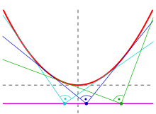
The orthoptic of a parabola is its directrix (proof: see below),
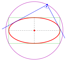
The orthoptic of an ellipse $x 2 / a 2 + y 2 / b 2 = 1$ is the director circle $x 2 + y 2 = a 2 + b 2$ (see below),
The orthoptic of a hyperbola $x 2 / a 2 - y 2 / b 2 = 1$ , $a > b$ , is the circle $x 2 + y 2 = a 2 - b 2$ (in case of $a \leq b$ there are no orthogonal tangents, see below),
The orthoptic of an astroid $x 2 ⁄ 3 + y 2 ⁄ 3 = 1$ is a quadrifolium with the polar equation

r={\tfrac {1}{\sqrt {2}}}\cos(2\varphi ),\quad 0\leq \varphi <2\pi

(see below).

Generalizations:

An isoptic is the set of points for which two tangents of a given curve meet at a fixed angle (see below).
An isoptic of two plane curves is the set of points for which two tangents meet at a fixed angle.
Thales' theorem on a chord $PQ$ can be considered as the orthoptic of two circles which are degenerated to the two points $P$ and $Q$ .

Orthoptic of a parabola

Any parabola can be transformed by a rigid motion (angles are not changed) into a parabola with equation $y=ax^{2}$ . The slope at a point of the parabola is $m=2ax$ . Replacing $x$ gives the parametric representation of the parabola with the tangent slope as parameter: $\ ({\tfrac {m}{2a}},{\tfrac {m^{2}}{4a}})\;.$ The tangent has the equation $y=mx+n$ with the still unknown $n$ , which can be determined by inserting the coordinates of the parabola point. One gets $\ y=mx-{\tfrac {m^{2}}{4a}}\;.$

If a tangent contains the point $(x 0, y 0)$ , off the parabola, then the equation

y_{0}=mx_{0}-{\frac {m^{2}}{4a}}\quad \rightarrow \quad m^{2}-4ax_{0}\;m+4ay_{0}=0

holds, which has two solutions $m 1$ and $m 2$ corresponding to the two tangents passing $(x 0, y 0)$ . The free term of a reduced quadratic equation is always the product of its solutions. Hence, if the tangents meet at $(x 0, y 0)$ orthogonally, the following equations hold:

m_{1}m_{2}=-1=4ay_{0}

The last equation is equivalent to

y_{0}=-{\frac {1}{4a}}\;,

which is the equation of the directrix.

Orthoptic of an ellipse and hyperbola

Ellipse

Let $\;E:\;{\tfrac {x^{2}}{a^{2}}}+{\tfrac {y^{2}}{b^{2}}}=1\;$ be the ellipse of consideration.

(1) The tangents of ellipse $E$ at neighbored vertices intersect at one of the 4 points $(\pm a,\pm b)$ , which lie on the desired orthoptic curve (circle $x^{2}+y^{2}=a^{2}+b^{2}$ ).

(2) The tangent at a point $(u,v)$ of the ellipse $E$ has the equation ${\tfrac {u}{a^{2}}}x+{\tfrac {v}{b^{2}}}y=1$ (s. Ellipse). If the point is not a vertex this equation can be solved: $\ y=-{\tfrac {b^{2}u}{a^{2}v}}\;x\;+\;{\tfrac {b^{2}}{v}}\;.$

Using the abbreviations $(I)\;m=-{\tfrac {b^{2}u}{a^{2}v}},\;{\color {red}n={\tfrac {b^{2}}{v}}}\;$ and the equation $\;{\color {blue}{\tfrac {u^{2}}{a^{2}}}=1-{\tfrac {v^{2}}{b^{2}}}=1-{\tfrac {b^{2}}{n^{2}}}}\;$ one gets:

m^{2}={\frac {b^{4}u^{2}}{a^{4}v^{2}}}={\frac {1}{a^{2}}}{\color {red}{\frac {b^{4}}{v^{2}}}}{\color {blue}{\frac {u^{2}}{a^{2}}}}={\frac {1}{a^{2}}}{\color {red}n^{2}}{\color {blue}(1-{\frac {b^{2}}{n^{2}}})}={\frac {n^{2}-b^{2}}{a^{2}}}\;.

Hence $\ (II)\;n=\pm {\sqrt {m^{2}a^{2}+b^{2}}}$ and the equation of a non vertical tangent is

y=m\;x\;\pm {\sqrt {m^{2}a^{2}+b^{2}}}.

Solving relations $(I)$ for $u,v$ and respecting $(II)$ leads to the slope depending parametric representation of the ellipse:

(u,v)=(-{\tfrac {ma^{2}}{\pm {\sqrt {m^{2}a^{2}+b^{2}}}}}\;,\;{\tfrac {b^{2}}{\pm {\sqrt {m^{2}a^{2}+b^{2}}}}})\ .\

(For an other proof: see Ellipse.)

If a tangent contains the point $(x_{0},y_{0})$ , off the ellipse, then the equation

y_{0}=mx_{0}\pm {\sqrt {m^{2}a^{2}+b^{2}}}

holds. Eliminating the square root leads to

m^{2}-{\frac {2x_{0}y_{0}}{x_{0}^{2}-a^{2}}}m+{\frac {y_{0}^{2}-b^{2}}{x_{0}^{2}-a^{2}}}=0,

which has two solutions $(x_{0},y_{0})$ corresponding to the two tangents passing $(x_{0},y_{0})$ . The free term of a reduced quadratic equation is always the product of its solutions. Hence, if the tangents meet at $(x_{0},y_{0})$ orthogonally, the following equations hold:

Orthoptics (red circles) of a circle, ellipses and hyperbolas

m_{1}m_{2}=-1={\frac {y_{0}^{2}-b^{2}}{x_{0}^{2}-a^{2}}}

The last equation is equivalent to

x_{0}^{2}+y_{0}^{2}=a^{2}+b^{2}\;.

From (1) and (2) one gets:

The intersection points of orthogonal tangents are points of the circle $x^{2}+y^{2}=a^{2}+b^{2}$ .

Hyperbola

The ellipse case can be adopted nearly exactly to the hyperbola case. The only changes to be made are to replace $b^{2}$ with $-b^{2}$ and to restrict $m$ to $| m | > b / a$ . Therefore:

The intersection points of orthogonal tangents are points of the circle $x^{2}+y^{2}=a^{2}-b^{2}$ , where $a > b$ .

Orthoptic of an astroid

Orthoptic (purple) of an astroid

An astroid can be described by the parametric representation

{\vec {c}}(t)=\left(\cos ^{3}t,\sin ^{3}t\right),\quad 0\leq t<2\pi

.

From the condition

{\vec {\dot c}}(t)\cdot {\vec {\dot c}}(t+\alpha )=0

one recognizes the distance $α$ in parameter space at which an orthogonal tangent to $ċ \to (t)$ appears. It turns out that the distance is independent of parameter $t$ , namely $α = \pm π / 2$ . The equations of the (orthogonal) tangents at the points $c \to (t)$ and $c \to (t + π / 2)$ are respectively:

{\begin{aligned}y&=-\tan t\left(x-\cos ^{3}t\right)+\sin ^{3}t,\\y&={\frac {1}{\tan t}}\left(x+\sin ^{3}t\right)+\cos ^{3}t.\end{aligned}}

Their common point has coordinates:

{\begin{aligned}x&=\sin t\cos t(\sin t-\cos t),\\y&=\sin t\cos t(\sin t+\cos t).\end{aligned}}

This is simultaneously a parametric representation of the orthoptic.

Elimination of the parameter $t$ yields the implicit representation

2\left(x^{2}+y^{2}\right)^{3}-\left(x^{2}-y^{2}\right)^{2}=0.

Introducing the new parameter $φ = t - 5π / 4$ one gets

{\begin{aligned}x&={\tfrac {1}{\sqrt {2}}}\cos(2\varphi )\cos \varphi ,\\y&={\tfrac {1}{\sqrt {2}}}\cos(2\varphi )\sin \varphi .\end{aligned}}

(The proof uses the angle sum and difference identities.) Hence we get the polar representation

r={\tfrac {1}{\sqrt {2}}}\cos(2\varphi ),\quad 0\leq \varphi <2\pi

of the orthoptic. Hence:

The orthoptic of an astroid is a quadrifolium.

Isoptic of a parabola, an ellipse and a hyperbola

Isoptics (purple) of a parabola for angles 80° and 100°

Isoptics (purple) of an ellipse for angles 80° and 100°

Isoptics (purple) of a hyperbola for angles 80° and 100°

Below the isotopics for angles $α \neq 90°$ are listed. They are called $α$ -isoptics. For the proofs see below.

Equations of the isoptics

Parabola:

The $α$ -isoptics of the parabola with equation $y = ax 2$ are the branches of the hyperbola

x^{2}-\tan ^{2}\alpha \left(y+{\frac {1}{4a}}\right)^{2}-{\frac {y}{a}}=0.

The branches of the hyperbola provide the isoptics for the two angles $α$ and $180° - α$ (see picture).

Ellipse:

The $α$ -isoptics of the ellipse with equation $x 2 / a 2 + y 2 / b 2 = 1$ are the two parts of the degree-4 curve

\left(x^{2}+y^{2}-a^{2}-b^{2}\right)^{2}\tan ^{2}\alpha =4\left(a^{2}y^{2}+b^{2}x^{2}-a^{2}b^{2}\right)

(see picture).

Hyperbola:

The $α$ -isoptics of the hyperbola with the equation $x 2 / a 2 - y 2 / b 2 = 1$ are the two parts of the degree-4 curve

\left(x^{2}+y^{2}-a^{2}+b^{2}\right)^{2}\tan ^{2}\alpha =4\left(a^{2}y^{2}-b^{2}x^{2}+a^{2}b^{2}\right).

Proofs

Parabola:

A parabola $y = ax 2$ can be parametrized by the slope of its tangents $m = 2 ax$ :

{\vec {c}}(m)=\left({\frac {m}{2a}},{\frac {m^{2}}{4a}}\right),\quad m\in \mathbb {R} .

The tangent with slope $m$ has the equation

y=mx-{\frac {m^{2}}{4a}}.

The point $(x 0, y 0)$ is on the tangent if and only if

y_{0}=mx_{0}-{\frac {m^{2}}{4a}}.

This means the slopes $m 1$ , $m 2$ of the two tangents containing $(x 0, y 0)$ fulfil the quadratic equation

m^{2}-4ax_{0}m+4ay_{0}=0.

If the tangents meet at angle $α$ or $180° - α$ , the equation

\tan ^{2}\alpha =\left({\frac {m_{1}-m_{2}}{1+m_{1}m_{2}}}\right)^{2}

must be fulfilled. Solving the quadratic equation for $m$ , and inserting $m 1$ , $m 2$ into the last equation, one gets

x_{0}^{2}-\tan ^{2}\alpha \left(y_{0}+{\frac {1}{4a}}\right)^{2}-{\frac {y_{0}}{a}}=0.

This is the equation of the hyperbola above. Its branches bear the two isoptics of the parabola for the two angles $α$ and $180° - α$ .

Ellipse:

In the case of an ellipse $x 2 / a 2 + y 2 / b 2 = 1$ one can adopt the idea for the orthoptic for the quadratic equation

m^{2}-{\frac {2x_{0}y_{0}}{x_{0}^{2}-a^{2}}}m+{\frac {y_{0}^{2}-b^{2}}{x_{0}^{2}-a^{2}}}=0.

Now, as in the case of a parabola, the quadratic equation has to be solved and the two solutions $m 1$ , $m 2$ must be inserted into the equation

\tan ^{2}\alpha =\left({\frac {m_{1}-m_{2}}{1+m_{1}m_{2}}}\right)^{2}.

Rearranging shows that the isoptics are parts of the degree-4 curve:

\left(x_{0}^{2}+y_{0}^{2}-a^{2}-b^{2}\right)^{2}\tan ^{2}\alpha =4\left(a^{2}y_{0}^{2}+b^{2}x_{0}^{2}-a^{2}b^{2}\right).

Hyperbola:

The solution for the case of a hyperbola can be adopted from the ellipse case by replacing $b 2$ with $- b 2$ (as in the case of the orthoptics, see above).

To visualize the isoptics, see implicit curve.

External links

Notes

References

Lawrence, J. Dennis (1972). A catalog of special plane curves. Dover Publications. pp. 58–59. ISBN 0-486-60288-5.
Odehnal, Boris (2010). "Equioptic Curves of Conic Sections". Journal for Geometry and Graphics. 14 (1): 29–43.
Schaal, Hermann (1977). "Lineare Algebra und Analytische Geometrie". III. Vieweg: 220. ISBN 3-528-03058-5.
Steiner, Jacob (1867). Vorlesungen über synthetische Geometrie. Leipzig: B. G. Teubner. Part 2, p. 186.
Ternullo, Maurizio (2009). "Two new sets of ellipse related concyclic points". Journal of Geometry. 94: 159–173.

This article is issued from Wikipedia. The text is licensed under Creative Commons - Attribution - Sharealike. Additional terms may apply for the media files.

Differential transforms of plane curves
Unary operations	Evolute Involute Dual curve Inverse curve Parallel curve Isoptic
Unary operations defined by a point	Pedal & Contrapedal curves Negative pedal curve Pursuit curve Caustic
Unary operations defined by two points	Strophoid
Binary operations defined by a point	Roulette Cissoid
Operations on a family of curves	Envelope