Newton's method in optimization
In calculus, Newton's method is an iterative method for finding the roots of a differentiable function f, which are solutions to the equation f (x) = 0. More specifically, in optimization, Newton's method is applied to the derivative f ′ of a twice-differentiable function f to find the roots of the derivative (solutions to f ′(x) = 0), also known as the stationary points of f. These solutions may be minima, maxima, or saddle points.
Method
In the one-dimensional problem, Newton's method attempts to find the roots of f ′ by constructing a sequence xn from an initial guess x0 that converges towards some value x* satisfying f ′(x*) = 0. This x* is a stationary point of f.
The second-order Taylor expansion fT (x) of a function f around xn is

Ideally, we want to pick a Δx such that xn + Δx is a stationary point of f. Using this Taylor expansion as an approximation, we can at least solve for the Δx corresponding to the root of the expansion's derivative:


Provided the Taylor approximation is fairly accurate, then incrementing by the above Δx should yield a point fairly close to an actual stationary point of f. This point, xn+1 = xn + Δx = xn − f ′(xn) / f ″(xn), we define to be the n + 1th guess in Newton's method; as n tends toward infinity, xn should approach a stationary point x* of the actual function f. Indeed, it is proven that if f is a twice-differentiable function and other technical conditions are satisfied, the sequence x1, x2, … will converge to a point x* satisfying f ′(x*) = 0.
Geometric interpretation
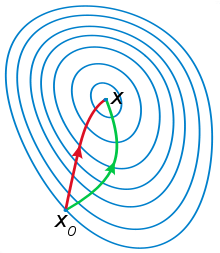
The geometric interpretation of Newton's method is that at each iteration, f (x) is approximated by a quadratic function around xn, and a step is taken to the maximum or minimum of that quadratic function (in higher dimensions, this may also be a saddle point). Note that if f (x) happens to be a quadratic function, then the exact extremum is found in one step.
Higher dimensions
The above iterative scheme can be generalized to several dimensions by replacing the derivative with the gradient, ∇f (x), and the reciprocal of the second derivative with the inverse of the Hessian matrix, H f (x). One obtains the iterative scheme
![\mathbf {x} _{n+1}=\mathbf {x} _{n}-[\mathbf {H} f(\mathbf {x} _{n})]^{-1}\nabla f(\mathbf {x} _{n}),\ n\geq 0.](../I/m/75802c220f63e636fda641fbe2c953ed656a2ee2.svg)
Often Newton's method is modified to include a small step size γ ∈ (0,1) instead of γ = 1
![\mathbf {x} _{n+1}=\mathbf {x} _{n}-\gamma [\mathbf {H} f(\mathbf {x} _{n})]^{-1}\nabla f(\mathbf {x} _{n}).](../I/m/d8b266ce1ac150b43acb59eca9abf45fc08a33db.svg)
This is often done to ensure that the Wolfe conditions are satisfied at each step xn → xn+1 of the iteration. For step sizes other than 1, the method is often referred to as the relaxed Newton's method.
Where applicable, Newton's method converges much faster towards a local maximum or minimum than gradient descent. In fact, every local minimum has a neighborhood N such that, if we start with x0 ∈ N, Newton's method with step size γ = 1 converges quadratically (if the Hessian is invertible and a Lipschitz continuous function of x in that neighborhood).
Finding the inverse of the Hessian in high dimensions can be an expensive operation. In such cases, instead of directly inverting the Hessian it's better to calculate the vector Δx = xn + 1 - xn as the solution to the system of linear equations
![[\mathbf {H} f(\mathbf {x} _{n})]\mathbf {\Delta x} =-\nabla f(\mathbf {x} _{n})](../I/m/c19002921fdd62924a8d1b07f3a1e196d6f3e3ec.svg)
which may be solved by various factorizations or approximately (but to great accuracy) using iterative methods. Many of these methods are only applicable to certain types of equations, for example the Cholesky factorization and conjugate gradient will only work if [H f(xn)] is a positive definite matrix. While this may seem like a limitation, it's often a useful indicator of something gone wrong; for example if a minimization problem is being approached and [H f(xn)] is not positive definite, then the iterations are converging to a saddle point and not a minimum.
On the other hand, if a constrained optimization is done (for example, with Lagrange multipliers), the problem may become one of saddle point finding, in which case the Hessian will be symmetric indefinite and the solution of xn+1 will need to be done with a method that will work for such, such as the LDLT variant of Cholesky factorization or the conjugate residual method.
There also exist various quasi-Newton methods, where an approximation for the Hessian (or its inverse directly) is built up from changes in the gradient.
If the Hessian is close to a non-invertible matrix, the inverted Hessian can be numerically unstable and the solution may diverge. In this case, certain workarounds have been tried in the past, which have varied success with certain problems. One can, for example, modify the Hessian by adding a correction matrix Bn so as to make Hf(xn) + Bn positive definite. One approach is to diagonalize H f(xn) and choose Bn so that H f(xn) + Bn has the same eigenvectors as H f(xn), but with each negative eigenvalue replaced by ϵ > 0.
An approach exploited in the Levenberg–Marquardt algorithm (which uses an approximate Hessian) is to add a scaled identity matrix to the Hessian, μI, with the scale adjusted at every iteration as needed. For large μ and small Hessian, the iterations will behave like gradient descent with step size 1 / μ. This results in slower but more reliable convergence where the Hessian doesn't provide useful information.
See also
Notes
References
- Avriel, Mordecai (2003). Nonlinear Programming: Analysis and Methods. Dover Publishing. ISBN 0-486-43227-0.
- Bonnans, J. Frédéric; Gilbert, J. Charles; Lemaréchal, Claude; Sagastizábal, Claudia A. (2006). Numerical optimization: Theoretical and practical aspects. Universitext (Second revised ed. of translation of 1997 French ed.). Berlin: Springer-Verlag. pp. xiv+490. doi:10.1007/978-3-540-35447-5. ISBN 3-540-35445-X. MR 2265882.
- Fletcher, Roger (1987). Practical methods of optimization (2nd ed.). New York: John Wiley & Sons. ISBN 978-0-471-91547-8.
- Nocedal, Jorge; Wright, Stephen J. (1999). Numerical Optimization. Springer-Verlag. ISBN 0-387-98793-2.
External links
- Korenblum, Daniel (Aug 29, 2015). "Newton-Raphson visualization (1D)". Bl.ocks. ffe9653768cb80dfc0da.
|  | |||||||||||||||||
|
| ||||||||||||||||||
| ||||||||||||||||||