Multigrid method
Multigrid (MG) methods in numerical analysis are algorithms for solving differential equations using a hierarchy of discretizations. They are an example of a class of techniques called multiresolution methods, very useful in problems exhibiting multiple scales of behavior. For example, many basic relaxation methods exhibit different rates of convergence for short- and long-wavelength components, suggesting these different scales be treated differently, as in a Fourier analysis approach to multigrid.[1] MG methods can be used as solvers as well as preconditioners.
The main idea of multigrid is to accelerate the convergence of a basic iterative method (known as relaxation, which generally reduces short-wavelength error) by a global correction of the fine grid solution approximation from time to time, accomplished by solving a coarse problem. The coarse problem, while cheaper to solve, is similar to the fine grid problem in that it also has short- and long-wavelength errors. It can also be solved by a combination of relaxation and appeal to still coarser grids. This recursive process is repeated until a grid is reached where the cost of direct solution there is negligible compared to the cost of one relaxation sweep on the fine grid. This multigrid cycle typically reduces all error components by a fixed amount bounded well below one, independent of the fine grid mesh size. The typical application for multigrid is in the numerical solution of elliptic partial differential equations in two or more dimensions.[2]
Multigrid methods can be applied in combination with any of the common discretization techniques. For example, the finite element method may be recast as a multigrid method.[3] In these cases, multigrid methods are among the fastest solution techniques known today. In contrast to other methods, multigrid methods are general in that they can treat arbitrary regions and boundary conditions. They do not depend on the separability of the equations or other special properties of the equation. They have also been widely used for more-complicated non-symmetric and nonlinear systems of equations, like the Lamé equations of elasticity or the Navier-Stokes equations.[4]
Algorithm
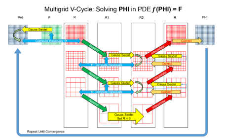
There are many variations of multigrid algorithms, but the common features are that a hierarchy of discretizations (grids) is considered. The important steps are:[5][6]
- Smoothing – reducing high frequency errors, for example using a few iterations of the Gauss–Seidel method.
- Restriction – downsampling the residual error to a coarser grid.
- Interpolation or prolongation – interpolating a correction computed on a coarser grid into a finer grid.
Computational cost
This approach has the advantage over other methods that it often scales linearly with the number of discrete nodes used. In other words, it can solve these problems to a given accuracy in a number of operations that is proportional to the number of unknowns.
Assume that one has a differential equation which can be solved approximately (with a given accuracy) on a grid with a given grid point density . Assume furthermore that a solution on any grid may be obtained with a given effort from a solution on a coarser grid . Here, is the ratio of grid points on "neighboring" grids and is assumed to be constant throughout the grid hierarchy, and is some constant modeling the effort of computing the result for one grid point.


The following recurrence relation is then obtained for the effort of obtaining the solution on grid :


And in particular, we find for the finest grid that


Combining these two expressions (and using ) gives


Using the geometric series, we then find (for finite )


that is, a solution may be obtained in time.

Multigrid preconditioning
A multigrid method with an intentionally reduced tolerance can be used as an efficient preconditioner for an external iterative solver. The solution may still be obtained in time as well as in the case where the multigrid method is used as a solver. Multigrid preconditioning is used in practice even for linear systems, typically with one cycle per iteration. Its main advantage versus a purely multigrid solver is particularly clear for nonlinear problems, e.g., eigenvalue problems.
Generalized multigrid methods
Multigrid methods can be generalized in many different ways. They can be applied naturally in a time-stepping solution of parabolic partial differential equations, or they can be applied directly to time-dependent partial differential equations.[7] Research on multilevel techniques for hyperbolic partial differential equations is underway.[8] Multigrid methods can also be applied to integral equations, or for problems in statistical physics.[9]
Other extensions of multigrid methods include techniques where no partial differential equation nor geometrical problem background is used to construct the multilevel hierarchy.[10] Such algebraic multigrid methods (AMG) construct their hierarchy of operators directly from the system matrix. In classical AMG, the levels of the hierarchy are simply subsets of unknowns without any geometric interpretation. (More generally, coarse grid unknowns can be particular linear combinations of fine grid unknowns.) Thus, AMG methods become black-box solvers for certain classes of sparse matrices. AMG is regarded as advantageous mainly where geometric multigrid is too difficult to apply,[11] but is often used simply because it avoids the coding necessary for a true multigrid implementation. While classical AMG was developed first, a related algebraic method is known as smoothed aggregation (SA).
Another set of multiresolution methods is based upon wavelets. These wavelet methods can be combined with multigrid methods.[12][13] For example, one use of wavelets is to reformulate the finite element approach in terms of a multilevel method.[14]
Adaptive multigrid exhibits adaptive mesh refinement, that is, it adjusts the grid as the computation proceeds, in a manner dependent upon the computation itself.[15] The idea is to increase resolution of the grid only in regions of the solution where it is needed.
Multigrid in time methods
Multigrid methods have also been adopted for the solution of initial value problems.[16] Of particular interest here are parallel-in-time multigrid methods:[17] in contrast to classical Runge-Kutta or linear multistep methods, they can offer concurrency in temporal direction. The well known Parareal parallel-in-time integration method can also be reformulated as a two-level multigrid in time.
Notes
- ↑ Roman Wienands; Wolfgang Joppich (2005). Practical Fourier analysis for multigrid methods. CRC Press. p. 17. ISBN 1-58488-492-4.
- ↑ U. Trottenberg; C. W. Oosterlee; A. Schüller (2001). Multigrid. Academic Press. ISBN 0-12-701070-X.
- ↑ Yu Zhu; Andreas C. Cangellaris (2006). Multigrid finite element methods for electromagnetic field modeling. Wiley. p. 132 ff. ISBN 0-471-74110-8.
- ↑ Shah, Tasneem Mohammad (1989). Analysis of the multigrid method (Thesis). Oxford University. Bibcode:1989STIN...9123418S.
- ↑ M. T. Heath (2002). "Section 11.5.7 Multigrid Methods". Scientific Computing: An Introductory Survey. McGraw-Hill Higher Education. p. 478 ff. ISBN 0-07-112229-X.
- ↑ P. Wesseling (1992). An Introduction to Multigrid Methods. Wiley. ISBN 0-471-93083-0.
- ↑ F. Hülsemann; M. Kowarschik; M. Mohr; U. Rüde (2006). "Parallel geometric multigrid". In Are Magnus Bruaset, Aslak Tveito. Numerical solution of partial differential equations on parallel computers. Birkhäuser. p. 165. ISBN 3-540-29076-1.
- ↑ For example, J. Blaz̆ek (2001). Computational fluid dynamics: principles and applications. Elsevier. p. 305. ISBN 0-08-043009-0. and Achi Brandt and Rima Gandlin (2003). "Multigrid for Atmospheric Data Assimilation: Analysis". In Thomas Y. Hou, Eitan Tadmor. Hyperbolic problems: theory, numerics, applications: proceedings of the Ninth International Conference on Hyperbolic Problems of 2002. Springer. p. 369. ISBN 3-540-44333-9.
- ↑ Achi Brandt (2002). "Multiscale scientific computation: review". In Timothy J. Barth, Tony Chan, Robert Haimes. Multiscale and multiresolution methods: theory and applications. Springer. p. 53. ISBN 3-540-42420-2.
- ↑ Yair Shapira (2003). "Algebraic multigrid". Matrix-based multigrid: theory and applications. Springer. p. 66. ISBN 1-4020-7485-9.
- ↑ U. Trottenberg; C. W. Oosterlee; A. Schüller. op. cit.. p. 417. ISBN 0-12-701070-X.
- ↑ Björn Engquist; Olof Runborg (2002). "Wavelet-based numerical homogenization with applications". In Timothy J. Barth, Tony Chan, Robert Haimes. Multiscale and Multiresolution Methods. Vol. 20 of Lecture Notes in Computational Science and Engineering. Springer. p. 140 ff. ISBN 3-540-42420-2.
- ↑ U. Trottenberg; C. W. Oosterlee; A. Schüller. op. cit.. ISBN 0-12-701070-X.
- ↑ Albert Cohen (2003). Numerical Analysis of Wavelet Methods. Elsevier. p. 44. ISBN 0-444-51124-5.
- ↑ U. Trottenberg; C. W. Oosterlee; A. Schüller. "Chapter 9: Adaptive Multigrid". op. cit.. p. 356. ISBN 0-12-701070-X.
- ↑ Hackbusch, Wolfgang (1985). "Parabolic multi-grid methods". Computing Methods in Applied Sciences and Engineering, VI. North-Holland Publishing Co: 189–197. Retrieved August 2015. Check date values in:
|access-date=(help) - ↑ Horton, Graham (1992). "The time-parallel multigrid method". Communications in Applied Numerical Methods. Wiley. 8 (9): 585–595. doi:10.1002/cnm.1630080906. Retrieved August 2015. Check date values in:
|access-date=(help)
References
- G. P. Astrachancev (1971), An iterative method of solving elliptic net problems. USSR Comp. Math. Math. Phys. 11, 171–182.
- N. S. Bakhvalov (1966), On the convergence of a relaxation method with natural constraints on the elliptic operator. USSR Comp. Math. Math. Phys. 6, 101–13.
- Achi Brandt (April 1977), "Multi-Level Adaptive Solutions to Boundary-Value Problems", Mathematics of Computation, 31: 333–90.
- William L. Briggs, Van Emden Henson, and Steve F. McCormick (2000), A Multigrid Tutorial (2nd ed.), Philadelphia: Society for Industrial and Applied Mathematics, ISBN 0-89871-462-1.
- R. P. Fedorenko (1961), A relaxation method for solving elliptic difference equations. USSR Comput. Math. Math. Phys. 1, p. 1092.
- R. P. Fedorenko (1964), The speed of convergence of one iterative process. USSR Comput. Math. Math. Phys. 4, p. 227.
- Press, W. H.; Teukolsky, S. A.; Vetterling, W. T.; Flannery, B. P. (2007). "Section 20.6. Multigrid Methods for Boundary Value Problems". Numerical Recipes: The Art of Scientific Computing (3rd ed.). New York: Cambridge University Press. ISBN 978-0-521-88068-8.