Mean time between failures

Mean time between failures (MTBF) is the predicted elapsed time between inherent failures of a mechanical or electronic system, during normal system operation. MTBF can be calculated as the arithmetic mean (average) time between failures of a system. The term is used for repairable systems, while mean time to failure (MTTF) denotes the expected time to failure for a non-repairable system.^[1]

The definition of MTBF depends on the definition of what is considered a failure. For complex, repairable systems, failures are considered to be those out of design conditions which place the system out of service and into a state for repair. Failures which occur that can be left or maintained in an unrepaired condition, and do not place the system out of service, are not considered failures under this definition.^[2] In addition, units that are taken down for routine scheduled maintenance or inventory control are not considered within the definition of failure.^[3] The higher the MTBF, the longer a system is likely to work before failing.

Overview

Mean time between failures (MTBF) describes the expected time between two failures for a repairable system. For example, three identical systems starting to function properly at time 0 are working until all of them fail. The first system failed at 100 hours, the second failed at 120 hours and the third failed at 130 hours. The MTBF of the system is the average of the three failure times, which is 116.667 hours. If the systems are non-repairable, then their MTTF would be 116.667 hours.

In general, MTBF is the "up-time" between two failure states of a repairable system during operation as outlined here:

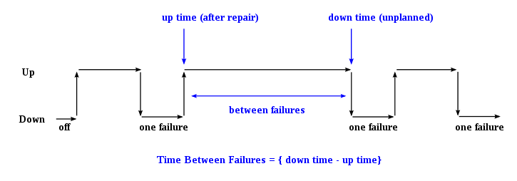
For each observation, the "down time" is the instantaneous time it went down, which is after (i.e. greater than) the moment it went up, the "up time". The difference ("down time" minus "up time") is the amount of time it was operating between these two events.

By referring to the figure above, the MTBF of a component is the sum of the lengths of the operational periods divided by the number of observed failures:

{\text{MTBF}}={\frac {\sum {({\text{start of downtime}}-{\text{start of uptime}})}}{\text{number of failures}}}.

In a similar manner, mean down time (MDT) can be defined as

{\text{MDT}}={\frac {\sum {({\text{start of uptime}}-{\text{start of downtime}})}}{\text{number of failures}}}.

Calculation

MTBF is defined by the arithmetic mean value of the reliability function R(t), which can be expressed as the expected value of the density function ƒ(t) of time until failure:^[4]

{\text{MTBF}}=\int _{0}^{\infty }R(t)\,dt=\int _{0}^{\infty }tf(t)\,dt

Any practically-relevant calculation of MTBF or probabilistic failure prediction based on MTBF requires that the system is working within its "useful life period", which is characterized by a relatively constant failure rate (the middle part of the "bathtub curve") when only random failures are occurring.^[1]

Assuming a constant failure rate results in a failure density function as follows: $f(t)=\lambda e^{-\lambda t}$ , which, in turn, simplifies the above mentioned calculation of MTBF to the reciprocal of the failure rate of the system^[1]^[4]

{\text{MTBF}}={\frac {1}{\lambda }}.\!

The units used are typically hours or lifecycles. This critical relationship between a system's MTBF and its failure rate allows a simple conversion/calculation when one of the two quantities is known and an exponential distribution (constant failure rate, i.e., no systematic failures) can be assumed.

Once the MTBF of a system is known, the probability that any one particular system will be operational at time equal to the MTBF can be estimated.^[1] Under the assumption of a constant failure rate, any one particular system will survive to its calculated MTBF with a probability of 36.8% (i.e., it will fail before with a probability of 63.2%).^[1] The same applies to the MTTF of a system working within this time period.^[5]

Application

The MTBF value can be used as a system reliability parameter or to compare different systems or designs. This value should only be understood conditionally as the “mean lifetime” (an average value), and not as a quantitative identity between working and failed units.^[1]

Since MTBF can be expressed as “average life (expectancy)”, many engineers assume that 50% of items will have failed by time t = MTBF. This inaccuracy can lead to bad design decisions. Furthermore, probabilistic failure prediction based on MTBF implies the total absence of systematic failures (i.e., a constant failure rate with only intrinsic, random failures), which is not easy to verify.^[4] Assuming no systematic errors, the probability of failure during a duration, T, is calculated as exp^(-T/MTBF).

MTBF value prediction is an important element in the development of products. Reliability engineers and design engineers often use reliability software to calculate a product's MTBF according to various methods and standards (MIL-HDBK-217F, Telcordia SR332, Siemens Norm, FIDES,UTE 80-810 (RDF2000), etc.). The Mil-HDBK-217 reliability calculator manual in combination with RelCalc software (or other comparable tool) enables MTBF reliability rates to be predicted based on design.

A concept which is closely related to MTBF, and is important in the computations involving MTBF, is the mean down time (MDT). MDT can be defined as mean time which the system is down after the failure. Usually, MDT is considered different from MTTR (Mean Time To Repair); in particular, MDT usually includes organizational and logistical factors (such as business days or waiting for components to arrive) while MTTR is usually understood as more narrow and more technical.

MTBF and MDT for networks of components

Two components $c_{1},c_{2}$ (for instance hard drives, servers, etc.) may be arranged in a network, in series or in parallel. The terminology is here used by close analogy to electrical circuits, but has a slightly different meaning. We say that the two components are in series if the failure of either causes the failure of the network, and that they are in parallel if only the failure of both causes the network to fail. The MTBF of the resulting two-component network with repairable components can be computed according to the following formulae, assuming that the MTBF of both individual components is known:^[6]^[7]

{\text{mtbf}}(c_{1};c_{2})={\frac {1}{{\frac {1}{{\text{mtbf}}(c_{1})}}+{\frac {1}{{\text{mtbf}}(c_{2})}}}}={\frac {{\text{mtbf}}(c_{1})\times {\text{mtbf}}(c_{2})}{{\text{mtbf}}(c_{1})+{\text{mtbf}}(c_{2})}}\;,

where $c_{1};c_{2}$ is the network in which the components are arranged in series.

For the network containing parallel repairable components, to find out the MTBF of the whole system, in addition to component MTBFs, it is also necessary to know their respective MDTs. Then, assuming that MDTs are negligible compared to MTBFs (which usually stands in practice), the MTBF for the parallel system consisting from two parallel repairable components can be written as follows:^[6]^[7]

${\begin{aligned}{\text{mtbf}}(c_{1}\parallel c_{2})&={\frac {1}{{\frac {1}{{\text{mtbf}}(c_{1})}}\times {\text{PF}}(c_{2},{\text{mdt}}(c_{1}))+{\frac {1}{{\text{mtbf}}(c_{2})}}\times {\text{PF}}(c_{1},{\text{mdt}}(c_{2}))}}\\[1em]&={\frac {1}{{\frac {1}{{\text{mtbf}}(c_{1})}}\times {\frac {{\text{mdt}}(c_{1})}{{\text{mtbf}}(c_{2})}}+{\frac {1}{{\text{mtbf}}(c_{2})}}\times {\frac {{\text{mdt}}(c_{2})}{{\text{mtbf}}(c_{1})}}}}\\[1em]&={\frac {{\text{mtbf}}(c_{1})\times {\text{mtbf}}(c_{2})}{{\text{mdt}}(c_{1})+{\text{mdt}}(c_{2})}}\;,\end{aligned}}$

where $c_{1}\parallel c_{2}$ is the network in which the components are arranged in parallel, and $PF(c,t)$ is the probability of failure of component $c$ during "vulnerability window" $t$ .

Intuitively, both these formulae can be explained from the point of view of failure probabilities. First of all, let's note that the probability of a system failing within a certain timeframe is the inverse of its MTBF. Then, when considering series of components, failure of any component leads to the failure of the whole system, so (assuming that failure probabilities are small, which is usually the case) probability of the failure of the whole system within a given interval can be approximated as a sum of failure probabilities of the components. With parallel components the situation is a bit more complicated: the whole system will fail if and only if after one of the components fails, the other component fails while the first component is being repaired; this is where MDT comes into play: the faster the first component is repaired, the less is the "vulnerability window" for the other component to fail.

Using similar logic, MDT for a system out of two serial components can be calculated as:^[6]

{\text{mdt}}(c_{1};c_{2})={\frac {{\text{mtbf}}(c_{1})\times {\text{mdt}}(c_{2})+{\text{mtbf}}(c_{2})\times {\text{mdt}}(c_{1})}{{\text{mtbf}}(c_{1})+{\text{mtbf}}(c_{2})}}\;,

and for a system out of two parallel components MDT can be calculated as:^[6]

{\text{mdt}}(c_{1}\parallel c_{2})={\frac {{\text{mdt}}(c_{1})\times {\text{mdt}}(c_{2})}{{\text{mdt}}(c_{1})+{\text{mdt}}(c_{2})}}\;.

Through successive application of these four formulae, the MTBF and MDT of any network of repairable components can be computed, provided that the MTBF and MDT is known for each component. In a special but all-important case of several serial components, MTBF calculation can be easily generalised into

{\text{mtbf}}(c_{1};\dots ;c_{n})=\left(\sum _{k=1}^{n}{\frac {1}{{\text{mtbf}}(c_{k})}}\right)^{-1}\;,

which can be shown by induction,^[8] and likewise

{\text{mdt}}(c_{1}\parallel \dots \parallel c_{n})=\left(\sum _{k=1}^{n}{\frac {1}{{\text{mdt}}(c_{k})}}\right)^{-1}\;,

since the formula for the mdt of two components in parallel is identical to that of the mtbf for two components in series.

Variations of MTBF

There are many variations of MTBF, such as mean time between system aborts (MTBSA), mean time between critical failures (MTBCF) or mean time between unscheduled removal (MTBUR). Such nomenclature is used when it is desirable to differentiate among types of failures, such as critical and non-critical failures. For example, in an automobile, the failure of the FM radio does not prevent the primary operation of the vehicle.

It is recommended to use Mean time to failure (MTTF) instead of MTBF in cases where a system is replaced after a failure ("non-repairable system"), since MTBF denotes time between failures in a system which can be repaired.^[1]

MTTFd is an extension of MTTF, where MTTFd is only concerned about failures which would result in a dangerous condition. It can be calculated as follows:

{\begin{aligned}{\text{MTTF}}&\approx {\frac {B_{10}}{0.1n_{\text{onm}}}},\\[8pt]{\text{MTTFd}}&\approx {\frac {B_{10d}}{0.1n_{\text{op}}}},\end{aligned}}

where B₁₀ is the number of operations that a device will operate prior to 10% of a sample of those devices would fail and n_op is number of operations. B_10d is the same calculation, but where 10% of the sample would fail to danger. n_op is the number of operations/cycles in one year.^[9]

References

1 2 3 4 5 6 7 J. Lienig, H. Bruemmer (2017). "Reliability Analysis". Fundamentals of Electronic Systems Design. Springer International Publishing. pp. 49–56. ISBN 978-3-319-55839-4.
↑ Colombo, A.G., and Sáiz de Bustamante, Amalio: Systems reliability assessment – Proceedings of the Ispra Course held at the Escuela Tecnica Superior de Ingenieros Navales, Madrid, Spain, September 19–23, 1988 in collaboration with Universidad Politecnica de Madrid, 1988
↑ "Defining Failure: What Is MTTR, MTTF, and MTBF?". Stephen Foskett, Pack Rat. Retrieved 2016-01-18.
1 2 3 Alessandro Birolini: Reliability Engineering: Theory and Practice. Springer, Berlin 2013, ISBN 978-3-642-39534-5.
↑ "Reliability and MTBF Overview" (PDF). Vicor Reliability Engineering. Retrieved 1 June 2017.
1 2 3 4 "Reliability Characteristics for Two Subsystems in Series or Parallel or n Subsystems in m_out_of_n Arrangement (by Don L. Lin)". auroraconsultingengineering.com.
1 2 Dr. David J. Smith. Reliability, Maintainability and Risk (eighth ed.). ISBN 978-0080969022.
↑ "MTBF Allocations Analysis1". www.angelfire.com. Retrieved 2016-12-23.
↑ "B10d Assessment – Reliability Parameter for Electro-Mechanical Components" (PDF). TUVRheinland. Retrieved 7 July 2015.

External links

"Reliability and Availability Basics". EventHelix.
Speaks, Scott (2005). "Reliability and MTBF Overview" (PDF). Vicor Reliability Engineering.
"Failure Rates, MTBF, and All That". MathPages.

This article is issued from Wikipedia. The text is licensed under Creative Commons - Attribution - Sharealike. Additional terms may apply for the media files.

[lienig-1] 1 2 3 4 5 6 7 J. Lienig, H. Bruemmer (2017). "Reliability Analysis". Fundamentals of Electronic Systems Design. Springer International Publishing. pp. 49–56. ISBN 978-3-319-55839-4.

[2] Colombo, A.G., and Sáiz de Bustamante, Amalio: Systems reliability assessment – Proceedings of the Ispra Course held at the Escuela Tecnica Superior de Ingenieros Navales, Madrid, Spain, September 19–23, 1988 in collaboration with Universidad Politecnica de Madrid, 1988

[3] "Defining Failure: What Is MTTR, MTTF, and MTBF?". Stephen Foskett, Pack Rat. Retrieved 2016-01-18.

[birolini-4] 1 2 3 Alessandro Birolini: Reliability Engineering: Theory and Practice. Springer, Berlin 2013, ISBN 978-3-642-39534-5.

[5] "Reliability and MTBF Overview" (PDF). Vicor Reliability Engineering. Retrieved 1 June 2017.

[auroraconsultingengineering-6] 1 2 3 4 "Reliability Characteristics for Two Subsystems in Series or Parallel or n Subsystems in m_out_of_n Arrangement (by Don L. Lin)". auroraconsultingengineering.com.

[smith-7] 1 2 Dr. David J. Smith. Reliability, Maintainability and Risk (eighth ed.). ISBN 978-0080969022.

[8] "MTBF Allocations Analysis1". www.angelfire.com. Retrieved 2016-12-23.

[9] "B10d Assessment – Reliability Parameter for Electro-Mechanical Components" (PDF). TUVRheinland. Retrieved 7 July 2015.