Linearization

In mathematics, linearization is finding the linear approximation to a function at a given point. In the study of dynamical systems, linearization is a method for assessing the local stability of an equilibrium point of a system of nonlinear differential equations or discrete dynamical systems.^[1] This method is used in fields such as engineering, physics, economics, and ecology.

Linearization of a function

Linearizations of a function are lines—usually lines that can be used for purposes of calculation. Linearization is an effective method for approximating the output of a function $y=f(x)$ at any $x=a$ based on the value and slope of the function at $x=b$ , given that $f(x)$ is differentiable on $[a,b]$ (or $[b,a]$ ) and that $a$ is close to $b$ . In short, linearization approximates the output of a function near $x=a$ .

For example, ${\sqrt {4}}=2$ . However, what would be a good approximation of ${\sqrt {4.001}}={\sqrt {4+.001}}$ ?

For any given function $y=f(x)$ , $f(x)$ can be approximated if it is near a known differentiable point. The most basic requisite is that $L_{a}(a)=f(a)$ , where $L_{a}(x)$ is the linearization of $f(x)$ at $x=a$ . The point-slope form of an equation forms an equation of a line, given a point $(H,K)$ and slope $M$ . The general form of this equation is: $y-K=M(x-H)$ .

Using the point $(a,f(a))$ , $L_{a}(x)$ becomes $y=f(a)+M(x-a)$ . Because differentiable functions are locally linear, the best slope to substitute in would be the slope of the line tangent to $f(x)$ at $x=a$ .

While the concept of local linearity applies the most to points arbitrarily close to $x=a$ , those relatively close work relatively well for linear approximations. The slope $M$ should be, most accurately, the slope of the tangent line at $x=a$ .

An approximation of f(x)=x^2 at (x, f(x))

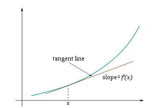
Visually, the accompanying diagram shows the tangent line of $f(x)$ at $x$ . At $f(x+h)$ , where $h$ is any small positive or negative value, $f(x+h)$ is very nearly the value of the tangent line at the point $(x+h,L(x+h))$ .

The final equation for the linearization of a function at $x=a$ is:

$y=(f(a)+f'(a)(x-a))$

For $x=a$ , $f(a)=f(x)$ . The derivative of $f(x)$ is $f'(x)$ , and the slope of $f(x)$ at $a$ is $f'(a)$ .

Example

To find ${\sqrt {4.001}}$ , we can use the fact that ${\sqrt {4}}=2$ . The linearization of $f(x)={\sqrt {x}}$ at $x=a$ is $y={\sqrt {a}}+{\frac {1}{2{\sqrt {a}}}}(x-a)$ , because the function $f'(x)={\frac {1}{2{\sqrt {x}}}}$ defines the slope of the function $f(x)={\sqrt {x}}$ at $x$ . Substituting in $a=4$ , the linearization at 4 is $y=2+{\frac {x-4}{4}}$ . In this case $x=4.001$ , so ${\sqrt {4.001}}$ is approximately $2+{\frac {4.001-4}{4}}=2.00025$ . The true value is close to 2.00024998, so the linearization approximation has a relative error of less than 1 millionth of a percent.

Linearization of a multivariable function

The equation for the linearization of a function $f(x,y)$ at a point $p(a,b)$ is:

$f(x,y)\approx f(a,b)+\left.{{\frac {{\partial f(x,y)}}{{\partial x}}}}\right|_{{a,b}}(x-a)+\left.{{\frac {{\partial f(x,y)}}{{\partial y}}}}\right|_{{a,b}}(y-b)$

The general equation for the linearization of a multivariable function $f(\mathbf {x} )$ at a point $\mathbf {p}$ is:

$f({{\mathbf {x}}})\approx f({{\mathbf {p}}})+\left.{\nabla f}\right|_{{{\mathbf {p}}}}\cdot ({{\mathbf {x}}}-{{\mathbf {p}}})$

where $\mathbf {x}$ is the vector of variables, and $\mathbf {p}$ is the linearization point of interest .^[2]

Uses of linearization

Linearization makes it possible to use tools for studying linear systems to analyze the behavior of a nonlinear function near a given point. The linearization of a function is the first order term of its Taylor expansion around the point of interest. For a system defined by the equation

{\frac {d{\mathbf {x}}}{dt}}={\mathbf {F}}({\mathbf {x}},t)

,

the linearized system can be written as

{\frac {d{\mathbf {x}}}{dt}}\approx {\mathbf {F}}({\mathbf {x_{0}}},t)+D{\mathbf {F}}({\mathbf {x_{0}}},t)\cdot ({\mathbf {x}}-{\mathbf {x_{0}}})

where ${\mathbf {x_{0}}}$ is the point of interest and $D{\mathbf {F}}({\mathbf {x_{0}}})$ is the Jacobian of ${\mathbf {F}}({\mathbf {x}})$ evaluated at ${\mathbf {x_{0}}}$ .

Stability analysis

In stability analysis of autonomous systems, one can use the eigenvalues of the Jacobian matrix evaluated at a hyperbolic equilibrium point to determine the nature of that equilibrium. This is the content of linearization theorem. For time-varying systems, the linearization requires additional justification.^[3]

Microeconomics

In microeconomics, decision rules may be approximated under the state-space approach to linearization.^[4] Under this approach, the Euler equations of the utility maximization problem are linearized around the stationary steady state.^[4] A unique solution to the resulting system of dynamic equations then is found.^[4]

Optimization

In mathematical optimization, cost functions and non-linear components within can be linearized in order to apply a linear solving method such as the Simplex algorithm. The optimized result is reached much more efficiently and is deterministic as a global optimum.

Multiphysics

In multiphysics systems — systems involving multiple physical fields that interact with one another — linearization with respect to each of the physical fields may be performed. This linearization of the system with respect to each of the fields results in a linearized monolithic equation system that can be solved using monolithic iterative solution procedures such as the Newton-Raphson method. Examples of this include MRI scanner systems which results in a system of electromagnetic, mechanical and acoustic fields.^[5]

References

↑ The linearization problem in complex dimension one dynamical systems at Scholarpedia
↑ Linearization. The Johns Hopkins University. Department of Electrical and Computer Engineering Archived 2010-06-07 at the Wayback Machine.
↑ G.A. Leonov, N.V. Kuznetsov, Time-Varying Linearization and the Perron effects, International Journal of Bifurcation and Chaos, Vol. 17, No. 4, 2007, pp. 1079-1107
1 2 3 Moffatt, Mike. (2008) About.com State-Space Approach Economics Glossary; Terms Beginning with S. Accessed June 19, 2008.
↑ S. Bagwell, P.D. Ledger, A.J. Gil, M. Mallett, M. Kruip, A linearised hp–finite element framework for acousto-magneto-mechanical coupling in axisymmetric MRI scanners, DOI: 10.1002/nme.5559

External links

Linearization tutorials

Linearization for Model Analysis and Control Design

This article is issued from Wikipedia. The text is licensed under Creative Commons - Attribution - Sharealike. Additional terms may apply for the media files.

[1] The linearization problem in complex dimension one dynamical systems at Scholarpedia

[2] Linearization. The Johns Hopkins University. Department of Electrical and Computer Engineering Archived 2010-06-07 at the Wayback Machine.

[3] G.A. Leonov, N.V. Kuznetsov, Time-Varying Linearization and the Perron effects, International Journal of Bifurcation and Chaos, Vol. 17, No. 4, 2007, pp. 1079-1107

[statespace-4] 1 2 3 Moffatt, Mike. (2008) About.com State-Space Approach Economics Glossary; Terms Beginning with S. Accessed June 19, 2008.

[5] S. Bagwell, P.D. Ledger, A.J. Gil, M. Mallett, M. Kruip, A linearised hp–finite element framework for acousto-magneto-mechanical coupling in axisymmetric MRI scanners, DOI: 10.1002/nme.5559