Lennard-Jones potential

A graph of strength versus distance for the 12-6 Lennard-Jones potential

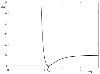
The Lennard-Jones potential (also termed the L-J potential, 6-12 potential, or 12-6 potential) is a mathematically simple model that approximates the interaction between a pair of neutral atoms or molecules. A form of this interatomic potential was first proposed in 1924 by John Lennard-Jones.^[1] The most common expressions of the L-J potential are

V_{\text{LJ}}=4\varepsilon \left[\left({\frac {\sigma }{r}}\right)^{12}-\left({\frac {\sigma }{r}}\right)^{6}\right]=\varepsilon \left[\left({\frac {r_{\text{m}}}{r}}\right)^{12}-2\left({\frac {r_{\text{m}}}{r}}\right)^{6}\right],

where ε is the depth of the potential well, σ is the finite distance at which the inter-particle potential is zero, r is the distance between the particles, and r_m is the distance at which the potential reaches its minimum. At r_m, the potential function has the value −ε. The distances are related as r_m = 2^1/6σ ≈ 1.122σ. These parameters can be fitted to reproduce experimental data or accurate quantum chemistry calculations. Due to its computational simplicity, the Lennard-Jones potential is used extensively in computer simulations even though more accurate potentials exist.

Explanation

The r⁻¹² term, which is the repulsive term, describes Pauli repulsion at short ranges due to overlapping electron orbitals, and the r⁻⁶ term, which is the attractive long-range term, describes attraction at long ranges (van der Waals force, or dispersion force).

Differentiating the L-J potential with respect to r gives an expression for the net inter-molecular force between 2 molecules. This inter-molecular force may be attractive or repulsive, depending on the value of r. When r is very small, the molecules repel each other.

Whereas the functional form of the attractive term has a clear physical justification, the repulsive term has no theoretical justification. It is used because it approximates the Pauli repulsion well and is more convenient due to the relative computing efficiency of calculating r¹² as the square of r⁶.

The L-J potential is a relatively good approximation. Due to its simplicity, it is often used to describe the properties of gases and to model dispersion and overlap interactions in molecular models. It is especially accurate for noble gas atoms and is a good approximation at long and short distances for neutral atoms and molecules.

The lowest-energy arrangement of an infinite number of atoms described by a Lennard-Jones potential is a hexagonal close-packing. On raising temperature, the lowest-free-energy arrangement becomes cubic close packing, and then liquid. Under pressure, the lowest-energy structure switches between cubic and hexagonal close packing.^[2] Real materials include body-centered cubic structures also.^[3]

The Lennard-Jones (12,6) potential was improved by the Buckingham potential (exp-6) later proposed by Richard Buckingham, incorporating an extra parameter and the repulsive part is replaced by an exponential function:^[4]

V_{\text{B}}=\gamma \left[e^{-r/r_{1}}-\left({\frac {r_{0}}{r}}\right)^{6}\right].

Other more recent methods, such as the Stockmayer potential, describe the interaction of molecules more accurately. Quantum chemistry methods, Møller–Plesset perturbation theory, coupled cluster method, or full configuration interaction can give extremely accurate results, but require large computing cost.

Alternative expressions

There are many different ways to formulate the Lennard-Jones potential. Some common forms follow.

AB form

This form is a simplified formulation that is used by some simulation software:

V_{\text{LJ}}(r)={\frac {A}{r^{12}}}-{\frac {B}{r^{6}}},

where, $A=4\varepsilon \sigma ^{12}$ and $B=4\varepsilon \sigma ^{6}$ . Conversely, $\sigma ={\sqrt[{6}]{\frac {A}{B}}}$ and $\varepsilon ={\frac {B^{2}}{4A}}$ . This is the form in which Lennard-Jones wrote the 12-6 potential.^[5]

A more mathematical general form, which contains an extra variable n is

V_{\text{LJ}}(r)=\varepsilon \left(\left({\frac {r_{0}}{r}}\right)^{2n}-2\left({\frac {r_{0}}{r}}\right)^{n}\right),

where $\varepsilon$ is the bonding energy of the molecule (the energy required to separate the atoms). The exponent n could be related to the spring constant k (at $r_{0}$ , where $V=-\varepsilon$ ) as

k=\varepsilon \left({\frac {n}{r_{0}}}\right)^{2},

from where n can be calculated if k is known. Normally the harmonic states are known, $\Delta E=\hbar \omega$ , where $\omega ={\sqrt {k/m}}$ . Also to the group velocity in a crystal, $v_{\text{g}}$

v_{\text{g}}={\frac {a\cdot n}{r_{0}}}{\sqrt {\frac {\varepsilon }{m}}},

where a is the lattice distance, and m is the mass of an atom.

Truncated and shifted form

To save computing time and satisfy the minimum image convention when using periodic boundary conditions, the Lennard-Jones potential is often truncated at a cut-off distance of r_c = 2.5σ, where

$\displaystyle V_{\text{LJ}}(r_{\text{c}})=V_{\text{LJ}}(2.5\sigma )=4\varepsilon \left[\left({\frac {\sigma }{2.5\sigma }}\right)^{12}-\left({\frac {\sigma }{2.5\sigma }}\right)^{6}\right]\approx -0.0163\varepsilon ,$

(1)

i.e., at r_c = 2.5σ, the Lennard-Jones potential V_LJ is about 1/60th of its minimum value, ε (the depth of the potential well). Beyond $r_{\text{c}}$ , the truncated potential is set to zero.

To avoid a jump discontinuity at $r_{\text{c}}$ , the LJ potential must be shifted upward a little, so that the truncated potential would be zero exactly at the cut-off distance, $r_{\text{c}}$ .

For clarity, let $V_{\text{LJ}}$ denote the LJ potential as defined above, i.e.,

$\displaystyle V_{\text{LJ}}(r)=4\varepsilon \left[\left({\frac {\sigma }{r}}\right)^{12}-\left({\frac {\sigma }{r}}\right)^{6}\right].$

(2)

Then the truncated Lennard-Jones potential $V_{{\text{LJ}}_{\text{trunc}}}$ is defined as follows^[6]

$\displaystyle V_{{\text{LJ}}_{\text{trunc}}}(r):={\begin{cases}V_{\text{LJ}}(r)-V_{\text{LJ}}(r_{\text{c}})&{\text{for }}r\leq r_{\text{c}}\\0&{\text{for }}r>r_{\text{c}}.\end{cases}}$

(3)

It can be easily verified that V_{LJ_trunc}(r_c) = 0, thus eliminating the jump discontinuity at r = r_c. Although the value of the (unshifted) Lennard Jones potential at r = r_c = 2.5σ is rather small, the effect of the truncation can be significant, for instance, on the gas–liquid critical point.^[7]^[8] The potential energy can often be corrected for this effect in a mean-field manner by adding so-called tail corrections.^[9]

Dimensionless (reduced) units

LJ dimensionless (reduced) units
Property	Symbol	Reduced form
Length	$r^{{*}}$	${\frac {r}{\sigma }}$
Time	$t^{*}$	${\frac {t}{\tau }}=t{\sqrt {\frac {\epsilon }{m\sigma ^{2}}}}$
Temperature	$T^{*}$	${\frac {k_{B}T}{\epsilon }}$
Force	$f^{*}$	${\frac {f\sigma }{\epsilon }}$
Energy	$\phi ^{*}$	${\frac {\phi }{\epsilon }}$
Pressure	$P^{*}$	${\frac {P\sigma ^{3}}{\epsilon }}$
Number density	$N^{*}$	$N\sigma ^{3}$
Density	$\rho^{*}$	$\rho \sigma ^{3}$
Surface tension	$\gamma ^{*}$	${\frac {\gamma \sigma ^{2}}{\epsilon }}$

Dimensionless units can be defined based on the Lennard-Jones potential, which are convenient for molecular dynamics simulations. From a numerical point, the advantages of dimensionless units include computing values which are closer to unity, using simplified equations and being able to easily scale the results.^[10]

When the Lennard-Jones potential is used for molecular dynamics simulations, the most convenient dimensionless units are obtained by choosing length σ, mass m and energy ε as the scaling factors for the various physical properties.^[10]

Limitations

The L-J potential has only two parameters (A and B), which determine the length and energy scales. The potential is therefore limited in how accurately it can be fitted to the properties of any real material.
With the L-J potential, the number of atoms bonded to an atom does not affect bond strength. The bond energy per atom thus rises linearly with the number of bonds per atom. But experiments show that in real materials, bond energy per atom rises quadratically with the number of bonds.^[11]
The bonding of the L-J potential has no directionality: the potential is spherically symmetric.
The sixth-power term models effectively the dipole–dipole interactions due to electron dispersion in noble gases (London dispersion forces), but it does not represent other kinds of bonding well. The twelfth-power term appearing in the potential is chosen for its ease of calculation for simulations (by squaring the sixth-power term) and is not theoretically or physically based.
The potential diverges when two atoms approach one another. This may create instabilities that require special treatment in molecular dynamics simulations.

References

↑ Lennard-Jones, J. E. (1924), "On the Determination of Molecular Fields", Proc. R. Soc. Lond. A, 106 (738): 463–477, Bibcode:1924RSPSA.106..463J, doi:10.1098/rspa.1924.0082
↑ Barron, T. H. K.; Domb, C. (1955), "On the Cubic and Hexagonal Close-Packed Lattices", Proceedings of the Royal Society of London. Series A, Mathematical and Physical Sciences, 227 (1171): 447–465, Bibcode:1955RSPSA.227..447B, doi:10.1098/rspa.1955.0023
↑ Zhen, Shu; Davies, G. J. (16 August 1983). "Calculation of the Lennard-Jones n–m potential energy parameters for metals". Physica Status Solidi A. 78 (2): 595–605.
↑ Peter Atkins and Julio de Paula, "Atkins' Physical Chemistry" (8th edn, W. H. Freeman), p. 637.
↑ Lennard-Jones, J. E. (1931). "Cohesion". Proceedings of the Physical Society. 43 (5): 461. Bibcode:1931PPS....43..461L. doi:10.1088/0959-5309/43/5/301.
↑ softmatter:Lennard-Jones Potential, Soft matter, Materials Digital Library Pathway, NIST-Lennard-Jones-fluid-properties.
↑ Smit, B. (1992), "Phase diagrams of Lennard-Jones fluids", Journal of Chemical Physics, 96 (11): 8639, Bibcode:1992JChPh..96.8639S, doi:10.1063/1.462271
↑ Di Pierro, M.; Elber, R.; Leimkuhler, B. (2015), "A Stochastic Algorithm for the Isobaric-Isothermal Ensemble with Ewald Summations for all Long Range Forces", Journal of Chemical Theory and Computation, doi:10.1021/acs.jctc.5b00648, PMC 4890727
↑ Frenkel, D. & Smit, B. (2002), Understanding Molecular Simulation (Second ed.), San Diego: Academic Press, ISBN 0-12-267351-4
1 2 D. C. Rapaport (1 April 2004). The Art of Molecular Dynamics Simulation. Cambridge University Press. ISBN 978-0-521-82568-9.
↑ Stachurski, Zbigniew H., Fundamentals of Amorphous Solids: Structure and Properties, p. 15

External links

This article is issued from Wikipedia. The text is licensed under Creative Commons - Attribution - Sharealike. Additional terms may apply for the media files.

[1] Lennard-Jones, J. E. (1924), "On the Determination of Molecular Fields", Proc. R. Soc. Lond. A, 106 (738): 463–477, Bibcode:1924RSPSA.106..463J, doi:10.1098/rspa.1924.0082

[2] Barron, T. H. K.; Domb, C. (1955), "On the Cubic and Hexagonal Close-Packed Lattices", Proceedings of the Royal Society of London. Series A, Mathematical and Physical Sciences, 227 (1171): 447–465, Bibcode:1955RSPSA.227..447B, doi:10.1098/rspa.1955.0023

[3] Zhen, Shu; Davies, G. J. (16 August 1983). "Calculation of the Lennard-Jones n–m potential energy parameters for metals". Physica Status Solidi A. 78 (2): 595–605.

[4] Peter Atkins and Julio de Paula, "Atkins' Physical Chemistry" (8th edn, W. H. Freeman), p. 637.

[LennardJones1931-5] Lennard-Jones, J. E. (1931). "Cohesion". Proceedings of the Physical Society. 43 (5): 461. Bibcode:1931PPS....43..461L. doi:10.1088/0959-5309/43/5/301.

[6] softmatter:Lennard-Jones Potential, Soft matter, Materials Digital Library Pathway, NIST-Lennard-Jones-fluid-properties.

[7] Smit, B. (1992), "Phase diagrams of Lennard-Jones fluids", Journal of Chemical Physics, 96 (11): 8639, Bibcode:1992JChPh..96.8639S, doi:10.1063/1.462271

[8] Di Pierro, M.; Elber, R.; Leimkuhler, B. (2015), "A Stochastic Algorithm for the Isobaric-Isothermal Ensemble with Ewald Summations for all Long Range Forces", Journal of Chemical Theory and Computation, doi:10.1021/acs.jctc.5b00648, PMC 4890727

[9] Frenkel, D. & Smit, B. (2002), Understanding Molecular Simulation (Second ed.), San Diego: Academic Press, ISBN 0-12-267351-4

[Rapaport2004-10] 1 2 D. C. Rapaport (1 April 2004). The Art of Molecular Dynamics Simulation. Cambridge University Press. ISBN 978-0-521-82568-9.

[11] Stachurski, Zbigniew H., Fundamentals of Amorphous Solids: Structure and Properties, p. 15