Orthogonal trajectory

Concentric circles with orthogonal trajectories (1. example)

Parabolas with orthogonal trajectories (2. example)

In mathematics an orthogonal trajectory is

a curve, which intersects any curve of a given pencil of (planar) curves orthogonally.

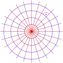
For example, the orthogonal trajectories of a pencil of concentric circles are the lines through their common center (see diagram).

Suitable methods for the determination of orthogonal trajectories are provided by solving differential equations. The standard method establishes a first order ordinary differential equation and solves it by separation of variables. Both steps may be difficult or even impossible. In such cases one has to apply numerical methods.

Orthogonal trajectories are used in mathematics for example as curved coordinate systems (i.e. elliptic coordinates) or appear in physics as electric fields and their equipotential curves.

If the trajectory intersects the given curves by an arbitrary (but fixed) angle, one gets an isogonal trajectory.

Determination of the orthogonal trajectory

In cartesian coordinates

Generally one assumes, that the pencil of curves is implicitly given by an equation

(0)

:\ F(x,y,c)=0,\qquad

1. example

:\ x^{2}+y^{2}-c=0\ ,\qquad

2. example

y=cx^{2}\ \leftrightarrow \ y-cx^{2}=0\ ,

where $c$ is the parameter of the pencil. If the pencil is given explicitly by an equation $y=f(x,c)$ , one can change the representation into an implicit one: $y-f(x,c)=0$ . For the consideration below it is supposed that all necessary derivatives do exist.

1. step

Differentiating implicitly for $x$ yields

(1) $:\ F_{x}(x,y,c)+F_{y}(x,y,c)\;y'=0,\qquad$ in 1. example $:\ 2x+2yy'=0\ ,\qquad$ 2. example $:\ y'-2cx=0\ .$
2. step

Now it is assumed, that equation (0) can be solved for parameter $c$ , which can thus be eliminated from equation (1). One gets the differential equation of first order

(2)

:\ y'=f(x,y),\qquad

in 1. example

:\ y'=-{\frac {x}{y}}\ ,\qquad

2. example

:\ y'=2{\frac {y}{x}}\ ,

which is fulfilled by the given pencil of curves.

3. step

Because the slope of the orthogonal trajectory at a point $(x,y)$ is the negative multiplicative inverse of the slope of the given curve at this point, the orthogonal trajectory satisfies the differential equation of first order

(3) $:\ y'=-{\frac {1}{f(x,y)}}\ ,\qquad$ in 1. example $:\ y'=y/x\ ,\qquad$ 2. example $:\ y'=-{\frac {x}{2y}}\ .$
4. step

This differential equation can (hopefully) be solved by a suitable method.
For both examples separation of variables is suitable. The solutions are:
in example 1, the lines $y=mx,\ m\in \mathbb {R}$ and
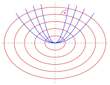
in example 2, the ellipses $x^{2}+2y^{2}=d,\ d>0\ .$

In polar coordinates

If the pencil of curves is represented implicitly in polar coordinates by

(0p)

:\ F(r,\varphi ,c)=0

one determines, alike the cartesian case, the parameter free differential equation

(1p)

:\ F_{r}(r,\varphi ,c)+F_{\varphi }(r,\varphi ,c)\;\varphi '=0,\qquad

(2p)

:\ \varphi '=f(r,\varphi )

of the pencil. The differential equation of the orthogonal trajectories is than (see Redheffer & Port p. 65, Heuser, p. 120)

(3p)

:\ \varphi '=-{\frac {1}{{\color {red}r^{2}}f(r,\varphi )}}\ .

Orthogonal cardioids

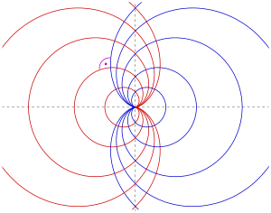
Example: Cardioids:

(0p)

:\ F(r,\varphi ,c)=r-c(1+\cos \varphi )=0,\ c>0\ .\

(in diagram: blue)

(1p)

:\ F_{r}(r,\varphi ,c)+F_{\varphi }(r,\varphi ,c)\;\varphi '=1+c\sin \varphi \;\varphi '=0,\qquad

Elimination of $c$ yields the differential equation of the given pencil:

(2p)

:\ \varphi '=-{\frac {1+\cos \varphi }{r\sin \varphi }}

Hence the differential equation of the orthogonal trajectories is:

(3p)

:\ \varphi '={\frac {\sin \varphi }{r(1+\cos \varphi )}}

After solving this differentialequation by separation of variables one gets

r=d(1-\cos \varphi )\ ,\ d>0\ ,

which describes the pencil of cardioids (red in diagram), symmetric to the given pencil.

Isogonal trajectory

A curve, which intersects any curve of a given pencil of (planar) curves by a fixed angle $\alpha$ is called isogonal trajectory.

Between the slope $\eta '$ of an isogonal trajectory and the slope $y'$ of the curve of the pencil at a point $(x,y)$ the following relation holds:

\eta '={\frac {y'+\tan(\alpha )}{1-y'\tan(\alpha )}}\ .

This relation is due to the formula for $\tan(\alpha +\beta )$ . For $\alpha \rightarrow 90^{\circ }$ one gets the condition for the orthogonal trajectory.

For the determination of the isogonal trajectory one has to adjust the 3. step of the instruction above:

3. step (isog. traj.)

The differential equation of the isogonal trajectory is:

(3i) $:\ y'={\frac {f(x,y)+\tan(\alpha )}{1-f(x,y)\;\tan(\alpha )}}\ .$

Isogonal trajectories of concentric circles for

\alpha =45^{\circ }

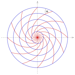
For the 1. example (concentric circles) and the angle $\alpha =45^{\circ }$ one gets

(3i)

:\ y'={\frac {-x/y+1}{1+x/y}}\ .

This is a special kind of differential equation, which can be transformed by the substitution $z=y/x$ into a differential equation, that can be solved by separation of variables. After reversing the substitution one gets the equation of the solution:

\arctan {\frac {y}{x}}+{\frac {1}{2}}\ln(x^{2}+y^{2})=C\ .

Introducing polar coordinates leads to the simple equation

C-\varphi =\ln(r)\ ,

which describes logarithmic spirals (s. diagram).

Numerical methods

In case that the differential equation of the trajectories can not be solved by theoretical methods, one has to solve it numerically, for example by Runge-Kutta methods.

References

A. Jeffrey: Advanced Engineering Mathematics, Hartcourt/Academic Press, 2002, ISBN 0-12-382592-X, p. 233.
S. B. Rao: Differential Equations, University Press, 1996, ISBN 81-7371-023-6, p. 95.
R. M. Redheffer, D. Port: Differential Equations: Theory and Applications, Jones & Bartlett, 1991, ISBN 0-86720-200-9, p. 63.
H. Heuser: Gewöhnliche Differentialgleichungen, Vieweg+Teubner, 2009, ISBN 978-3-8348-0705-2, p. 120.
Tenenbaum, Morris; Pollard, Harry (2012), Ordinary Differential Equations, Dover Books on Mathematics, Courier Dover, p. 115, ISBN 9780486134642 .

External links

Exploring orthogonal trajectories - applet allowing user to draw families of curves and their orthogonal trajectories.
mathcurve: FIELD LINES, ORTHOGONAL LINES, DOUBLE ORTHOGONAL SYSTEM

This article is issued from Wikipedia. The text is licensed under Creative Commons - Attribution - Sharealike. Additional terms may apply for the media files.