Incremental deformations

In solid mechanics, the linear stability analysis of an elastic solution is studied using the method of incremental deformations superposed on finite deformations.^[1] The method of incremental deformation can be used to solve static,^[2] quasi-static ^[3] and time-dependent problems.^[4] The governing equations of the motion are ones of the classical mechanics, such as the conservation of mass and the balance of linear and angular momentum, which provide the equilibrium configuration of the material.^[5] The main corresponding mathematical framework is described in the main Raymond Ogden's book Non-linear elastic deformations^[1] and in Biot's book Mechanics of incremental deformations,^[6] which is a collection of his main papers.

Nonlinear Elasticity

Kinematics and Mechanics

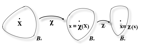
Scheme of the incremental deformation

Let ${\mathcal {E}}\in \mathbb {R} ^{3}$ be a three-dimensional Euclidean space. Let ${\mathcal {B}}_{0},{\mathcal {B}}_{a}\in {\mathcal {E}}$ be two regions occupied by the material in two different instants of time. Let ${\bf {\chi }}$ be the deformation which transforms the tissue from ${\mathcal {B}}_{0}$ , i.e. the material/reference configuration, to the loaded configuration ${\mathcal {B}}_{a}$ , i.e. current configuration. Let $\chi$ be a $C^{1}$ -diffeomorphism^[7] from ${\mathcal {B}}_{0}$ to ${\mathcal {B}}_{a}$ , with ${\bf {x}}={\bf {\chi }}({\bf {X}})$ being the current position vector, given as a function of the material position ${\bf {X}}$ . The deformation gradient^[5] is given by

${\bf {F}}={\rm {Grad}}\,{\bf {x}}={\frac {\partial {\bf {\chi }}({\bf {X)}}}{\partial {\bf {X}}}}$ .

Considering a hyperelastic material with an elastic strain energy density^[5] $W({\bf {F}})$ , the Piola-Kirchhoff stress tensor ${\bf {S}}$ is given by ${\bf {S}}={\frac {\partial W}{\partial \,{\bf {F}}}}$ .

For a quasi-static problem, without body forces, the equilibrium equation is

{\begin{aligned}{\rm {Div}}\,{\bf {S}}&=0&&\qquad {\text{Equilibrium}},\\[3pt]\end{aligned}}

where ${\rm {Div}}$ is the divergence^[1] with respect to the material coordinates.

If the material is incompressible,^[8] i.e. the volume of every subdomains does not change during the deformation, a Lagrangian multiplier^[9] is typically introduced to enforce the internal isochoric constraint ${\rm {det}}\,{\bf {F}}=1$ . So that, the expression of the Piola stress tensor becomes

{\begin{aligned}{\bf {S}}&={\frac {\partial W}{\partial {\bf {F}}}}-p{\bf {F}}^{-1}&&\qquad {\text{Definition of the stress}}.\\\end{aligned}}

Boundary conditions

Let $\partial {\mathcal {B}}_{0}$ be the boundary of ${\mathcal {B}}_{0}$ , the reference configuration, and $\partial {\mathcal {B}}_{a}$ , the boundary of ${\mathcal {B}}_{a}$ , the current configuration.^[1] One defines the subset $\Gamma _{D}$ of $\partial {\mathcal {B}}_{0}$ on which Dirichlet conditions are applied, while Neumann conditions hold on $\Gamma _{N}$ , such that $\partial {\mathcal {B}}_{0}=\Gamma _{D}\cup \Gamma _{N}$ . If ${\bf {u}}_{0}^{*}$ is the displacement vector to be assigned at the portion $\Gamma _{D}$ and ${\bf {t}}_{0}^{*}$ is the traction vector to be assigned to the portion $\Gamma _{N}$ , the boundary conditions can be written in mixed-form, such as

{\begin{aligned}{\bf {u}}({\bf {{X})}}&={\bf {u}}_{0}^{*}&&\qquad {\rm {on}}\,\Gamma _{D},\\[3pt]{\bf {S}}^{\rm {T}}\cdot {\bf {N}}&={\bf {t}}_{0}^{*}&&\qquad {\rm {on}}\,\Gamma _{N},\\[3pt]\end{aligned}}

where ${\bf {u}}={\bf {x}}-{\bf {X}}=\chi ({\bf {X}})-{\bf {X}}$ is the displacement and the vector ${\bf {N}}$ is the unit outward normal to $\partial {\mathcal {B}}_{0}$ .

Basic solution

The defined problem is called the boundary value problem (BVP). Hence, let ${\bf {x}}^{0}=\chi ^{0}({\bf {X}})$ be a solution of the BVP. Since $W$ depends nonlinearly^[10] on the deformation gradient, this solution is generally not unique, and it depends on geometrical and material parameters of the problem. So, one has to emply the method of incremental deformation in order to highlight the existence of an adiacent solution for a critical value of a dimensionless parameter, called control parameter $\gamma$ which "controls" the onset of the instability.^[11] This means that by increasing the value of this parameter, at a certain point new solutions appear. Hence, the selected basic solution is not anymore the stable one but it becomes unstable. In a physical way, at a certain time the stored energy, such as the integral of the density $W$ over all the domain of the basic solution is bigger than the one of the new solutions. To restore the equilibrium, the configuration of the material moves to another configuration which has lower energy.^[12]

Method of incremental deformations superposed on finite deformations

To improve this method, one has to superpose a small displacement $\delta {\bf {x}}$ on the finite deformation basic solution ${\bf {x}}^{0}$ . So that:

{\bar {\bf {x}}}={\bf {x}}^{0}+\delta {\bf {x}}={\bf {x}}^{0}+\chi ^{1}({\bf {x}}^{0})

,

where ${\bar {\bf {x}}}$ is the perturbed position and $\chi ^{1}({\bf {x}}^{0})$ maps the basic position vector ${\bf {x}}^{0}$ in the perturbed configuration $\delta {\mathcal {B}}_{a}$ .

In the following, the incremental variables are indicated by $\delta (\bullet )$ , while the perturbed ones are indicated by ${\bar {\bullet }}$ .^[1]

Deformation gradient

The perturbed deformation gradient is given by:

{\bar {\bf {F}}}={\bf {F}}^{0}+\delta {\bf {F}}=({\mathbf {I}}+{\mathbf {\Gamma }}){\bf {F}}^{0}

,

where ${\mathbf {\Gamma }}={\rm {grad}}\,\chi ^{1}({\bf {x}}^{0})$ , where ${\rm {grad}}$ is the gradient operator with respect to the actual configuration.

Stresses

The perturbed Piola stress is given by:

{\bar {\bf {S}}}={\bf {S}}^{0}+\delta {\bf {S}}={\bf {S}}^{0}+{\frac {\partial {\bf {S}}^{0}}{\partial {\bf {F}}}}{\bigg |}_{{\bf {F}}^{0}}:\delta {\bf {F}}

where $:$ denotes the contraction between two tensors, a forth-order tensor ${\frac {\partial {\bf {S}}^{0}}{\partial {\bf {F}}}}{\bigg |}_{{\bf {F}}^{0}}={\mathcal {A}}^{1}$ and a second-order tensor $\delta {\bf {F}}$ . Since ${\bf {S}}$ depends on ${\bf {F}}$ through $W$ , its expression can be rewritten by emphasizing this dependence, such as

${\bar {\bf {S}}}={\frac {\partial W}{\partial {\bf {F}}}}{\bigg |}_{{\bf {F}}^{0}}+{\frac {\partial W}{\partial {\bf {F}}\partial {\bf {F}}}}{\bigg |}_{{\bf {F}}^{0}}:\delta {\bf {F}}.$

If the material is incompressible, one gets

$\delta {\bf {S}}={\frac {\partial {\bf {S}}^{0}}{\partial {\bf {F}}}}\delta {\bf {F}}={\mathcal {A}}^{1}\delta {\bf {F}}+p({\bf {F}}^{0})^{-1}\delta {\bf {F}}-\delta p\,({\bf {F}}^{0})^{-1},$

where $\delta p$ is the increment in $p$ and ${\mathcal {A}}^{1}$ is called the elastic moduli associated to the pairs $({\bf {S}},{\bf {F}})$ .

It is useful to derive the push-forward of the perturbed Piola stress be defined as

\delta {\bf {S}}_{0}={\bf {F}}^{0}\,\delta {\bf {S}}={\mathcal {A}}_{0}^{1}\Gamma +p\,\delta {\bf {F}}-\delta p\,{\rm {I}},

where ${\mathcal {A}}_{0}^{1}$ is also known as the tensor of instantaneous moduli, whose components are:

({\mathcal {A}}_{0}^{1})_{ijhk}={\bf {F}}_{i\gamma }^{0}\,{\bf {F}}_{h\beta }^{0}\,{\mathcal {A}}_{\gamma j\beta k}^{1}

.

Incremental governing equations

Expanding the equilibrium equation around the basic solution, one gets

{\rm {Div}}({\bar {\bf {S}}})={\rm {Div}}({\bf {S}}^{0}+\delta {\bf {S}})={\rm {Div}}({\bf {S}}^{0})+\,{\rm {Div}}(\delta {\bf {S}})=0.

Since ${\bf {S}}^{0}$ is the solution to the equation at the zero-order, the incremental equation can be rewritten as

{\rm {div}}(\delta {\bf {S}}_{0})=0,

where ${\rm {div}}$ is the divergence operator with respect to the actual configuration.

The incremental incompressibility constraint reads

{\begin{aligned}{\rm {det}}\,({\bf {F}}^{0}+\delta {\bf {F}})&=1.\\\end{aligned}}

Expanding this equation around the basic solution, as before, one gets

{\rm {tr}}({\mathbf {\Gamma }})=0.

Incremental boundary conditions

Let ${\overline {\delta {\bf {u}}}}$ and ${\overline {\delta {\bf {t}}}}$ be the prescribed increment of ${\bf {u}}_{0}^{*}$ and ${\bf {t}}_{0}^{*}$ respectively. Hence, the perturbed boundary condition are

{\begin{aligned}\delta {\bf {u}}({\bf {x}})&={\overline {\delta {\bf {u}}}}&&\qquad {\bf {x}}\in {\Gamma _{D}}\\[3pt]\delta {\bf {S}}_{0}^{\rm {T}}\cdot {\bf {n}}&={\overline {\delta {\bf {t}}}}&&\qquad {\bf {x}}\in {\Gamma _{N}},\\[3pt]\end{aligned}}

where $\delta {\bf {u}}=\chi ^{1}({\bf {x}}^{0})-{\bf {x}}$ is the incremental displacement and ${\Gamma _{D}}\cup {\Gamma _{N}}={\partial \Omega }$ .

Solution of the incremental problem

The incremental equations

${\rm {div}}(\delta {\bf {S}}_{0})=0\qquad {\hbox{for compressible material}}$

${\begin{aligned}{\begin{cases}{\rm {div}}(\delta {\bf {S}}_{0})&=0\\{\rm {tr}}({\mathbf {\Gamma }})&=0\end{cases}}\qquad {\hbox{for incompressible material}}\end{aligned}}$

represent the incremental boundary value problem (BVP) and define a system of partial differential equations (PDEs).^[13] The unknowns of the problem depend on the considered case. For the first one, such as the compressible case, there are three unknowns, such as the components of the incremental deformations $\delta {u}_{1}({\bf {x}}),\delta {u}_{2}({\bf {x}}),\delta {u}_{3}({\bf {x}})$ , linked to the perturbed deformation by this relation $\chi ^{1}({\bf {x}})=\delta {u}_{1}({\bf {x}}){\bf {e}}_{1}+\delta {u}_{2}({\bf {x}}){\bf {e}}_{2}+\delta {u}_{3}({\bf {x}}){\bf {e}}_{3}$ . For the latter case, instead, one has to take into account also the increment $\delta p$ of the Lagrange multiplier $p$ , introduced to impose the isochoric constraint.

The main difficulty to solve this problem is to transform the problem in a more suitable form for implementing an effcient and robusted numerical solution procedure.^[14] The one used in this area is the Stroh formalism. It was originally developed by Stroh ^[15] for a steady state elastic problem and allows the set of four PDEs with the associated boundary conditions to be transformed into a set of ODEs of first order with initial conditions. The number of equtions depends on the dimension of the space in which the problem is set. To do this, one has to apply variable separation and assume periodicity in a given direction depending on the considered situation.^[16] In particular cases, the system can be rewritten in a compact form by using the Stroh formalism.^[15] Indeed, the shape of the system looks like

${\frac {d}{d\,{\rm {x}}}}{\eta }={\mathbf {G}}\,\eta ,$

where $\eta$ is the vector which contains all the unknowns of the problem, ${\rm {x}}$ is the only variable on which the rewritten problem depends and the matrix ${\bf {G}}$ is so-called Stroh matrix and it has the following form

{\bf {G}}={{\begin{bmatrix}{\bf {G}}_{1}&{\bf {G}}_{2}\\{\bf {G}}_{3}&{\bf {G}}_{4}\end{bmatrix}},}

where each block is a matrix and its dimension depends on the dimension of the problem. Moreover, a crucial property of this approach is that ${\bf {G}}_{4}=({\bf {G}}_{1})^{*}$ , i.e. ${\bf {G}}_{4}$ is the hermitian matrix of ${\bf {G}}_{1}$ .^[17]

Conclusion and remark

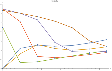
Result of the linear stability analysis.

The Stroh formalism provides an optimal form to solve a great variety of elastic problems. Optimal means that one can construct an efficient numerical procedure to solve the incremental problem. By solving the incremental boundary value problem, one finds the relations^[18] among the material and geometrical parameters of the problem and the perturbation modes by which the wave propagates in the material, i.e. what denotes the instability. Everything depends on $\gamma$ , the selected parameter denoted as the control one.

By this analysis, in a graph perturbation mode vs control parameter, the minimum value of the perturbation mode represents the first mode at which one can see the onset of the instability. For instance, in the picture, the first value of the mode $kz$ in which the instability emerges is around $0.3$ since the trivial solution $\gamma =0$ and $kz=0$ does not have to be considered.

References

1 2 3 4 5 Ogden, R. W. (1997). Non-linear elastic deformations (Corr. ed.). Mineola, N.Y.: Dover. ISBN 0486696480.
↑ Mora, Serge (2010). "Capillarity Driven Instability of a Soft Solid". Physical Review Letters. 105 (21). doi:10.1103/PhysRevLett.105.214301.
↑ Holzapfel, G. A.; Ogden, R. W. (31 March 2010). "Constitutive modelling of arteries". Proceedings of the Royal Society A: Mathematical, Physical and Engineering Sciences. 466 (2118): 1551–1597. doi:10.1098/rspa.2010.0058.
↑ Gower, A.L.; Destrade, M.; Ogden, R.W. (December 2013). "Counter-intuitive results in acousto-elasticity". Wave Motion. 50 (8): 1218–1228. doi:10.1016/j.wavemoti.2013.03.007.
1 2 3 Gurtin, Morton E. (1995). An introduction to continuum mechanics (6th [Dr.]. ed.). San Diego [u.a.]: Acad. Press. ISBN 9780123097507.
↑ Biot, M.A. (April 2009). "XLIII". The London, Edinburgh, and Dublin Philosophical Magazine and Journal of Science. 27 (183): 468–489. doi:10.1080/14786443908562246.
↑ 1921-2010., Rudin, Walter, (1991). Functional analysis (2nd ed.). New York: McGraw-Hill. ISBN 0070542368. OCLC 21163277.
↑ Horgan, C. O.; Murphy, J. G. (2018-03-01). "Magic angles for fibrous incompressible elastic materials". Proc. R. Soc. A. 474 (2211): 20170728. doi:10.1098/rspa.2017.0728. ISSN 1364-5021.
↑ Bertsekas, Dimitri P. (1996). Constrained optimization and Lagrange multiplier methods. Belmont, Mass.: Athena Scientific. ISBN 1-886529--04-3.
↑ Ball, John M. (December 1976). "Convexity conditions and existence theorems in nonlinear elasticity". Archive for Rational Mechanics and Analysis. 63 (4): 337–403. doi:10.1007/BF00279992.
↑ Levine, Howard A. (May 1974). "Instability and Nonexistence of Global Solutions to Nonlinear Wave Equations of the Form Pu tt = -Au + ℱ(u)". Transactions of the American Mathematical Society. 192: 1. doi:10.2307/1996814.
↑ Reid, L.D. Landau and E.M. Lifshitz ; translated from the Russian by J.B. Sykes and W.H. (1986). Theory of elasticity (3rd English ed., rev. and enl. by E.M. Lifshitz, A.M. Kosevich, and L.P. Pitaevskii. ed.). Oxford [England]: Butterworth-Heinemann. ISBN 9780750626330.
↑ Evans, Lawrence C. (2010). Partial differential equations (2nd ed.). Providence, R.I.: American Mathematical Society. ISBN 978-0821849743.
↑ Quarteroni, Alfio (2014). Numerical models for differential problems (Second edition. ed.). Milano: Springer Milan. ISBN 978-88-470-5522-3.
1 2 Stroh, A. N. (April 1962). "Steady State Problems in Anisotropic Elasticity". Journal of Mathematics and Physics. 41 (1–4): 77–103. doi:10.1002/sapm196241177.
↑ Destrade, M.; Ogden, R.W.; Sgura, I.; Vergori, L. (April 2014). "Straightening wrinkles". Journal of the Mechanics and Physics of Solids. 65: 1–11. doi:10.1016/j.jmps.2014.01.001.
↑ 1961-, Zhang, Fuzhen, (2011). Matrix theory : basic results and techniques (2nd ed.). New York: Springer. ISBN 9781461410997. OCLC 756201359.
↑ Ní Annaidh, Aisling; Bruyère, Karine; Destrade, Michel; Gilchrist, Michael D.; Maurini, Corrado; Otténio, Melanie; Saccomandi, Giuseppe (2012-03-17). "Automated Estimation of Collagen Fibre Dispersion in the Dermis and its Contribution to the Anisotropic Behaviour of Skin". Annals of Biomedical Engineering. 40 (8): 1666–1678. arXiv:1203.4733. doi:10.1007/s10439-012-0542-3. ISSN 0090-6964.

This article is issued from Wikipedia. The text is licensed under Creative Commons - Attribution - Sharealike. Additional terms may apply for the media files.

[ogden1-1] 1 2 3 4 5 Ogden, R. W. (1997). Non-linear elastic deformations (Corr. ed.). Mineola, N.Y.: Dover. ISBN 0486696480.

[2] Mora, Serge (2010). "Capillarity Driven Instability of a Soft Solid". Physical Review Letters. 105 (21). doi:10.1103/PhysRevLett.105.214301.

[ogden2-3] Holzapfel, G. A.; Ogden, R. W. (31 March 2010). "Constitutive modelling of arteries". Proceedings of the Royal Society A: Mathematical, Physical and Engineering Sciences. 466 (2118): 1551–1597. doi:10.1098/rspa.2010.0058.

[michel1-4] Gower, A.L.; Destrade, M.; Ogden, R.W. (December 2013). "Counter-intuitive results in acousto-elasticity". Wave Motion. 50 (8): 1218–1228. doi:10.1016/j.wavemoti.2013.03.007.

[gurtin1-5] 1 2 3 Gurtin, Morton E. (1995). An introduction to continuum mechanics (6th [Dr.]. ed.). San Diego [u.a.]: Acad. Press. ISBN 9780123097507.

[biot-6] Biot, M.A. (April 2009). "XLIII". The London, Edinburgh, and Dublin Philosophical Magazine and Journal of Science. 27 (183): 468–489. doi:10.1080/14786443908562246.

[7] 1921-2010., Rudin, Walter, (1991). Functional analysis (2nd ed.). New York: McGraw-Hill. ISBN 0070542368. OCLC 21163277.

[8] Horgan, C. O.; Murphy, J. G. (2018-03-01). "Magic angles for fibrous incompressible elastic materials". Proc. R. Soc. A. 474 (2211): 20170728. doi:10.1098/rspa.2017.0728. ISSN 1364-5021.

[lagrangian-9] Bertsekas, Dimitri P. (1996). Constrained optimization and Lagrange multiplier methods. Belmont, Mass.: Athena Scientific. ISBN 1-886529--04-3.

[ball-10] Ball, John M. (December 1976). "Convexity conditions and existence theorems in nonlinear elasticity". Archive for Rational Mechanics and Analysis. 63 (4): 337–403. doi:10.1007/BF00279992.

[instability-11] Levine, Howard A. (May 1974). "Instability and Nonexistence of Global Solutions to Nonlinear Wave Equations of the Form Pu tt = -Au + ℱ(u)". Transactions of the American Mathematical Society. 192: 1. doi:10.2307/1996814.

[landau-12] Reid, L.D. Landau and E.M. Lifshitz ; translated from the Russian by J.B. Sykes and W.H. (1986). Theory of elasticity (3rd English ed., rev. and enl. by E.M. Lifshitz, A.M. Kosevich, and L.P. Pitaevskii. ed.). Oxford [England]: Butterworth-Heinemann. ISBN 9780750626330.

[evans-13] Evans, Lawrence C. (2010). Partial differential equations (2nd ed.). Providence, R.I.: American Mathematical Society. ISBN 978-0821849743.

[alfio-14] Quarteroni, Alfio (2014). Numerical models for differential problems (Second edition. ed.). Milano: Springer Milan. ISBN 978-88-470-5522-3.

[stroh-15] 1 2 Stroh, A. N. (April 1962). "Steady State Problems in Anisotropic Elasticity". Journal of Mathematics and Physics. 41 (1–4): 77–103. doi:10.1002/sapm196241177.

[michel-16] Destrade, M.; Ogden, R.W.; Sgura, I.; Vergori, L. (April 2014). "Straightening wrinkles". Journal of the Mechanics and Physics of Solids. 65: 1–11. doi:10.1016/j.jmps.2014.01.001.

[17] 1961-, Zhang, Fuzhen, (2011). Matrix theory : basic results and techniques (2nd ed.). New York: Springer. ISBN 9781461410997. OCLC 756201359.

[18] Ní Annaidh, Aisling; Bruyère, Karine; Destrade, Michel; Gilchrist, Michael D.; Maurini, Corrado; Otténio, Melanie; Saccomandi, Giuseppe (2012-03-17). "Automated Estimation of Collagen Fibre Dispersion in the Dermis and its Contribution to the Anisotropic Behaviour of Skin". Annals of Biomedical Engineering. 40 (8): 1666–1678. arXiv:1203.4733. doi:10.1007/s10439-012-0542-3. ISSN 0090-6964.