Gaussian process

In probability theory and statistics, a Gaussian process is a stochastic process (a collection of random variables indexed by time or space), such that every finite collection of those random variables has a multivariate normal distribution, i.e. every finite linear combination of them is normally distributed. The distribution of a Gaussian process is the joint distribution of all those (infinitely many) random variables, and as such, it is a distribution over functions with a continuous domain, e.g. time or space.

A machine-learning algorithm that involves a Gaussian process uses lazy learning and a measure of the similarity between points (the kernel function) to predict the value for an unseen point from training data. The prediction is not just an estimate for that point, but also has uncertainty information—it is a one-dimensional Gaussian distribution (which is the marginal distribution at that point).^[1]

For some kernel functions, matrix algebra can be used to calculate the predictions using the technique of kriging. When a parameterised kernel is used, optimisation software is typically used to fit a Gaussian process model.

The concept of Gaussian processes is named after Carl Friedrich Gauss because it is based on the notion of the Gaussian distribution (normal distribution). Gaussian processes can be seen as an infinite-dimensional generalization of multivariate normal distributions.

Gaussian processes are useful in statistical modelling, benefiting from properties inherited from the normal. For example, if a random process is modelled as a Gaussian process, the distributions of various derived quantities can be obtained explicitly. Such quantities include the average value of the process over a range of times and the error in estimating the average using sample values at a small set of times.

Definition

A time continuous stochastic process is Gaussian if and only if for every finite set of indices $t_{1},\ldots ,t_{k}$ in the index set $T$

\mathbf {X} _{t_{1},\ldots ,t_{k}}=(\mathbf {X} _{t_{1}},\ldots ,\mathbf {X} _{t_{k}})

is a multivariate Gaussian random variable.^[2] That is the same as saying every linear combination of $(\mathbf {X} _{t_{1}},\ldots ,\mathbf {X} _{t_{k}})$ has a univariate normal (or Gaussian) distribution. Using characteristic functions of random variables, the Gaussian property can be formulated as follows: $\left\{X_{t};t\in T\right\}$ is Gaussian if and only if, for every finite set of indices $t_{1},\ldots ,t_{k}$ , there are real-valued $\sigma _{\ell j}$ , $\mu _{\ell }$ with $\sigma _{jj}>0$ such that the following equality holds for all $s_{1},s_{2},\ldots ,s_{k}\in \mathbb {R}$

\operatorname {E} \left(\exp \left(i\ \sum _{\ell =1}^{k}s_{\ell }\ \mathbf {X} _{t_{\ell }}\right)\right)=\exp \left(-{\frac {1}{2}}\,\sum _{\ell ,j}\sigma _{\ell j}s_{\ell }s_{j}+i\sum _{\ell }\mu _{\ell }s_{\ell }\right).

where $i$ denotes the imaginary unit ${\sqrt {-1}}$ .

The numbers $\sigma _{\ell j}$ and $\mu _{\ell }$ can be shown to be the covariances and means of the variables in the process.^[3]

Covariance functions

A key fact of Gaussian processes is that they can be completely defined by their second-order statistics.^[4] Thus, if a Gaussian process is assumed to have mean zero, defining the covariance function completely defines the process' behaviour. Importantly the non-negative definiteness of this function enables its spectral decomposition using the Karhunen–Loève expansion. Basic aspects that can be defined through the covariance function are the process' stationarity, isotropy, smoothness and periodicity.^[5]^[6]

Stationarity refers to the process' behaviour regarding the separation of any two points x and x' . If the process is stationary, it depends on their separation, x − x', while if non-stationary it depends on the actual position of the points x and x'. For example, the special case of an Ornstein–Uhlenbeck process, a Brownian motion process, is stationary.

If the process depends only on |x − x'|, the Euclidean distance (not the direction) between x and x', then the process is considered isotropic. A process that is concurrently stationary and isotropic is considered to be homogeneous;^[7] in practice these properties reflect the differences (or rather the lack of them) in the behaviour of the process given the location of the observer.

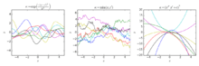
Ultimately Gaussian processes translate as taking priors on functions and the smoothness of these priors can be induced by the covariance function.^[5] If we expect that for "near-by" input points x and x' their corresponding output points y and y' to be "near-by" also, then the assumption of continuity is present. If we wish to allow for significant displacement then we might choose a rougher covariance function. Extreme examples of the behaviour is the Ornstein–Uhlenbeck covariance function and the squared exponential where the former is never differentiable and the latter infinitely differentiable.

Periodicity refers to inducing periodic patterns within the behaviour of the process. Formally, this is achieved by mapping the input x to a two dimensional vector u(x) = (cos(x), sin(x)).

Usual covariance functions

The effect of choosing different kernels on the prior function distribution of the Gaussian process. Left is a squared exponential kernel. Middle is Brownian. Right is quadratic.

There are a number of common covariance functions:^[6]

Constant : $K_{\operatorname {C} }(x,x')=C$
Linear: $K_{\operatorname {L} }(x,x')=x^{T}x'$
Gaussian noise: $K_{\operatorname {GN} }(x,x')=\sigma ^{2}\delta _{x,x'}$
Squared exponential: $K_{\operatorname {SE} }(x,x')=\exp {\Big (}-{\frac {\|d\|^{2}}{2\ell ^{2}}}{\Big )}$
Ornstein–Uhlenbeck: $K_{\operatorname {OU} }(x,x')=\exp \left(-{\frac {|d|}{\ell }}\right)$
Matérn: $K_{\operatorname {Matern} }(x,x')={\frac {2^{1-\nu }}{\Gamma (\nu )}}{\Big (}{\frac {{\sqrt {2\nu }}|d|}{\ell }}{\Big )}^{\nu }K_{\nu }{\Big (}{\frac {{\sqrt {2\nu }}|d|}{\ell }}{\Big )}$
Periodic: $K_{\operatorname {P} }(x,x')=\exp \left(-{\frac {2\sin ^{2}\left({\frac {d}{2}}\right)}{\ell ^{2}}}\right)$
Rational quadratic: $K_{\operatorname {RQ} }(x,x')=(1+|d|^{2})^{-\alpha },\quad \alpha \geq 0$

Here $d=x-x'$ . The parameter ℓ is the characteristic length-scale of the process (practically, "how close" two points $x$ and $x'$ have to be to influence each other significantly), δ is the Kronecker delta and σ the standard deviation of the noise fluctuations. Moreover, $K_{\nu }$ is the modified Bessel function of order $\nu$ and $\Gamma (\nu )$ is the gamma function evaluated at $\nu$ . Importantly, a complicated covariance function can be defined as a linear combination of other simpler covariance functions in order to incorporate different insights about the data-set at hand.

Clearly, the inferential results are dependent on the values of the hyperparameters θ (e.g. ℓ and σ) defining the model's behaviour. A popular choice for θ is to provide maximum a posteriori (MAP) estimates of it with some chosen prior. If the prior is very near uniform, this is the same as maximizing the marginal likelihood of the process; the marginalization being done over the observed process values $y$ .^[6] This approach is also known as maximum likelihood II, evidence maximization, or empirical Bayes.^[8]

Brownian motion as the integral of Gaussian processes

A Wiener process (aka Brownian motion) is the integral of a white noise Gaussian process. It is not stationary, but it has stationary increments.

The Ornstein–Uhlenbeck process is a stationary Gaussian process.

The Brownian bridge is (like the Ornstein–Uhlenbeck process) an example of a Gaussian process whose increments are not independent.

The fractional Brownian motion is a Gaussian process whose covariance function is a generalisation of that of the Wiener process.

Applications

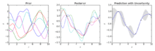
An example of Gaussian Process Regression (prediction) compared with other regression models.^[9]

A Gaussian process can be used as a prior probability distribution over functions in Bayesian inference.^[6]^[10] Given any set of N points in the desired domain of your functions, take a multivariate Gaussian whose covariance matrix parameter is the Gram matrix of your N points with some desired kernel, and sample from that Gaussian.

Inference of continuous values with a Gaussian process prior is known as Gaussian process regression, or kriging; extending Gaussian process regression to multiple target variables is known as cokriging.^[11] Gaussian processes are thus useful as a powerful non-linear multivariate interpolation tool. Gaussian process regression can be further extended to address learning tasks in both supervised (e.g. probabilistic classification^[6]) and unsupervised (e.g. manifold learning^[4]) learning frameworks.

Gaussian processes can also be used in the context of mixture of experts models, for example.^[12]^[13] The underlying rationale of such a learning framework consists in the assumption that a given mapping cannot be well captured by a single Gaussian process model. Instead, the observation space is divided into subsets, each of which is characterized by a different mapping function; each of these is learned via a different Gaussian process component in the postulated mixture.

Gaussian process prediction, or kriging

Gaussian Process Regression (prediction) with a squared exponential kernel. Left plot are draws from the prior function distribution. Middle are draws from the posterior. Right is mean prediction with one standard deviation shaded.

When concerned with a general Gaussian process regression problem (kriging), it is assumed that for a Gaussian process f observed at coordinates x, the vector of values $f(x)$ is just one sample from a multivariate Gaussian distribution of dimension equal to number of observed coordinates |x|. Therefore, under the assumption of a zero-mean distribution, $f(x)\sim N(0,K(\theta ,x,x'))$ , where $K(\theta ,x,x')$ is the covariance matrix between all possible pairs $(x,x')$ for a given set of hyperparameters θ.^[6] As such the log marginal likelihood is:

\log p(f(x)|\theta ,x)=-{\frac {1}{2}}f(x)^{T}K(\theta ,x,x')^{-1}f(x)-{\frac {1}{2}}\log \det(K(\theta ,x,x'))-{\frac {|x|}{2}}\log 2\pi

and maximizing this marginal likelihood towards θ provides the complete specification of the Gaussian process f. One can briefly note at this point that the first term corresponds to a penalty term for a model's failure to fit observed values and the second term to a penalty term that increases proportionally to a model's complexity. Having specified θ making predictions about unobserved values $f(x^{*})$ at coordinates x* is then only a matter of drawing samples from the predictive distribution $p(y^{*}\mid x^{*},f(x),x)=N(y^{*}\mid A,B)$ where the posterior mean estimate A is defined as

A=K(\theta ,x^{*},x)K(\theta ,x,x')^{-1}f(x)

and the posterior variance estimate B is defined as:

B=K(\theta ,x^{*},x^{*})-K(\theta ,x^{*},x)K(\theta ,x,x')^{-1}K(\theta ,x^{*},x)^{T}

where $K(\theta ,x^{*},x)$ is the covariance between the new coordinate of estimation x* and all other observed coordinates x for a given hyperparameter vector θ, $K(\theta ,x,x')$ and $f(x)$ are defined as before and $K(\theta ,x^{*},x^{*})$ is the variance at point x* as dictated by θ. It is important to note that practically the posterior mean estimate $f(x^{*})$ (the "point estimate") is just a linear combination of the observations $f(x)$ ; in a similar manner the variance of $f(x^{*})$ is actually independent of the observations $f(x)$ . A known bottleneck in Gaussian process prediction is that the computational complexity of prediction is cubic in the number of points |x| and as such can become unfeasible for larger data sets.^[5] Works on sparse Gaussian processes, that usually are based on the idea of building a representative set for the given process f, try to circumvent this issue.^[14]^[15]

Notes

↑ "Platypus Innovation: A Simple Intro to Gaussian Processes (a great data modelling tool)".
↑ MacKay, David, J.C. (2003). Information Theory, Inference, and Learning Algorithms (PDF). Cambridge University Press. p. 540. ISBN 9780521642989. The probability distribution of a function $y(\mathbf {x} )$ is a Gaussian processes if for any finite selection of points $\mathbf {x} ^{(1)},\mathbf {x} ^{(2)},\ldots ,\mathbf {x} ^{(N)}$ , the density $P(y(\mathbf {x} ^{(1)}),y(\mathbf {x} ^{(2)}),\ldots ,y(\mathbf {x} ^{(N)}))$ is a Gaussian
↑ Dudley, R.M. (1989). Real Analysis and Probability. Wadsworth and Brooks/Cole.
1 2 Bishop, C.M. (2006). Pattern Recognition and Machine Learning. Springer. ISBN 0-387-31073-8.
1 2 3 Barber, David (2012). Bayesian Reasoning and Machine Learning. Cambridge University Press. ISBN 978-0-521-51814-7.
1 2 3 4 5 6 Rasmussen, C.E.; Williams, C.K.I (2006). Gaussian Processes for Machine Learning. MIT Press. ISBN 0-262-18253-X.
↑ Grimmett, Geoffrey; David Stirzaker (2001). Probability and Random Processes. Oxford University Press. ISBN 0198572220.
↑ Seeger, Matthias (2004). "Gaussian Processes for Machine Learning". International Journal of Neural Systems. 14 (2): 69–104. doi:10.1142/s0129065704001899.
↑ The documentation for scikit-learn also has similar examples.
↑ Liu, W.; Principe, J.C.; Haykin, S. (2010). Kernel Adaptive Filtering: A Comprehensive Introduction. John Wiley. ISBN 0-470-44753-2.
↑ Stein, M.L. (1999). Interpolation of Spatial Data: Some Theory for Kriging. Springer.
↑ Emmanouil A. Platanios and Sotirios P. Chatzis, “Gaussian Process-Mixture Conditional Heteroscedasticity,” IEEE Transactions on Pattern Analysis and Machine Intelligence, vol. 36, no. 5, pp. 888–900, May 2014.
↑ Sotirios P. Chatzis, “A Latent Variable Gaussian Process Model with Pitman-Yor Process Priors for Multiclass Classification,” Neurocomputing, vol. 120, pp. 482–489, Nov. 2013.
↑ Smola, A.J.; Schoellkopf, B. (2000). "Sparse greedy matrix approximation for machine learning". Proceedings of the Seventeenth International Conference on Machine Learning: 911–918.
↑ Csato, L.; Opper, M. (2002). "Sparse on-line Gaussian processes". Neural Computation. 14 (3): 641–668. doi:10.1162/089976602317250933.

External links

Software

STK: a Small (Matlab/Octave) Toolbox for Kriging and GP modeling
Kriging module in UQLab framework (Matlab)
Matlab/Octave function for stationary Gaussian fields
Yelp MOE – A black box optimization engine using Gaussian process learning
ooDACE – A flexible object-oriented Kriging matlab toolbox.
GPstuff – Gaussian process toolbox for Matlab and Octave
GPy – A Gaussian processes framework in Python
Interactive Gaussian process regression demo
Basic Gaussian process library written in C++11
scikit-learn – A machine learning library for Python which includes Gaussian process regression and classification
- The Kriging toolKit (KriKit) is developed at the Institute of Bio- and Geosciences 1 (IBG-1) of Forschungszentrum Jülich (FZJ)

Video tutorials

This article is issued from Wikipedia. The text is licensed under Creative Commons - Attribution - Sharealike. Additional terms may apply for the media files.

[1] "Platypus Innovation: A Simple Intro to Gaussian Processes (a great data modelling tool)".

[DrMacKayGPNN-2] MacKay, David, J.C. (2003). Information Theory, Inference, and Learning Algorithms (PDF). Cambridge University Press. p. 540. ISBN 9780521642989. The probability distribution of a function $y(\mathbf {x} )$ is a Gaussian processes if for any finite selection of points $\mathbf {x} ^{(1)},\mathbf {x} ^{(2)},\ldots ,\mathbf {x} ^{(N)}$ , the density $P(y(\mathbf {x} ^{(1)}),y(\mathbf {x} ^{(2)}),\ldots ,y(\mathbf {x} ^{(N)}))$ is a Gaussian

[3] Dudley, R.M. (1989). Real Analysis and Probability. Wadsworth and Brooks/Cole.

[prml-4] 1 2 Bishop, C.M. (2006). Pattern Recognition and Machine Learning. Springer. ISBN 0-387-31073-8.

[brml-5] 1 2 3 Barber, David (2012). Bayesian Reasoning and Machine Learning. Cambridge University Press. ISBN 978-0-521-51814-7.

[gpml-6] 1 2 3 4 5 6 Rasmussen, C.E.; Williams, C.K.I (2006). Gaussian Processes for Machine Learning. MIT Press. ISBN 0-262-18253-X.

[PRP-7] Grimmett, Geoffrey; David Stirzaker (2001). Probability and Random Processes. Oxford University Press. ISBN 0198572220.

[seegerGPML-8] Seeger, Matthias (2004). "Gaussian Processes for Machine Learning". International Journal of Neural Systems. 14 (2): 69–104. doi:10.1142/s0129065704001899.

[9] The documentation for scikit-learn also has similar examples.

[10] Liu, W.; Principe, J.C.; Haykin, S. (2010). Kernel Adaptive Filtering: A Comprehensive Introduction. John Wiley. ISBN 0-470-44753-2.

[11] Stein, M.L. (1999). Interpolation of Spatial Data: Some Theory for Kriging. Springer.

[12] Emmanouil A. Platanios and Sotirios P. Chatzis, “Gaussian Process-Mixture Conditional Heteroscedasticity,” IEEE Transactions on Pattern Analysis and Machine Intelligence, vol. 36, no. 5, pp. 888–900, May 2014.

[13] Sotirios P. Chatzis, “A Latent Variable Gaussian Process Model with Pitman-Yor Process Priors for Multiclass Classification,” Neurocomputing, vol. 120, pp. 482–489, Nov. 2013.

[smolaSparse-14] Smola, A.J.; Schoellkopf, B. (2000). "Sparse greedy matrix approximation for machine learning". Proceedings of the Seventeenth International Conference on Machine Learning: 911–918.

[CsatoSparse-15] Csato, L.; Opper, M. (2002). "Sparse on-line Gaussian processes". Neural Computation. 14 (3): 641–668. doi:10.1162/089976602317250933.

Stochastic processes
Discrete time	Bernoulli process Branching process Chinese restaurant process Galton–Watson process Independent and identically distributed random variables Markov chain Moran process Random walk Loop-erased Self-avoiding Biased Maximal entropy
Continuous time	Bessel process Birth–death process Brownian motion Bridge Excursion Fractional Geometric Meander Cauchy process Contact process Continuous-time random walk Cox process Diffusion process Empirical process Feller process Fleming–Viot process Gamma process Hunt process Interacting particle systems Itô diffusion Itô process Jump diffusion Jump process Lévy process Local time Markov additive process McKean–Vlasov process Ornstein–Uhlenbeck process Poisson process Compound Non-homogeneous Point process Schramm–Loewner evolution Semimartingale Sigma-martingale Stable process Superprocess Telegraph process Variance gamma process Wiener process Wiener sausage
Both	Branching process Galves–Löcherbach model Gaussian process Hidden Markov model (HMM) Markov process Martingale Differences Local Sub- Super- Random dynamical system Regenerative process Renewal process Stochastic chains with memory of variable length White noise
Fields and other	Dirichlet process Gaussian random field Gibbs measure Hopfield model Ising model Potts model Boolean network Markov random field Percolation Pitman–Yor process Point process Cox Poisson Random field Random graph
Time series models	Autoregressive conditional heteroskedasticity (ARCH) model Autoregressive integrated moving average (ARIMA) model Autoregressive (AR) model Autoregressive–moving-average (ARMA) model Generalized autoregressive conditional heteroskedasticity (GARCH) model Moving-average (MA) model
Financial models	Black–Derman–Toy Black–Karasinski Black–Scholes Chen Constant elasticity of variance (CEV) Cox–Ingersoll–Ross (CIR) Garman–Kohlhagen Heath–Jarrow–Morton (HJM) Heston Ho–Lee Hull–White LIBOR market Rendleman–Bartter SABR volatility Vašíček Wilkie
Actuarial models	Bühlmann Cramér–Lundberg Risk process Sparre–Anderson
Queueing models	Bulk Fluid Generalized queueing network M/G/1 M/M/1 M/M/c
Properties	Càdlàg paths Continuous Continuous paths Ergodic Exchangeable Feller-continuous Gauss–Markov Markov Mixing Piecewise deterministic Predictable Progressively measurable Self-similar Stationary Time-reversible
Limit theorems	Central limit theorem Donsker's theorem Doob's martingale convergence theorems Ergodic theorem Fisher–Tippett–Gnedenko theorem Large deviation principle Law of large numbers (weak/strong) Law of the iterated logarithm Maximal ergodic theorem Sanov's theorem
Inequalities	Burkholder–Davis–Gundy Doob's martingale Kunita–Watanabe
Tools	Cameron–Martin formula Convergence of random variables Doléans-Dade exponential Doob decomposition theorem Doob–Meyer decomposition theorem Doob's optional stopping theorem Dynkin's formula Feynman–Kac formula Filtration Girsanov theorem Infinitesimal generator Itô integral Itô's lemma Kolmogorov continuity theorem Kolmogorov extension theorem Lévy–Prokhorov metric Malliavin calculus Martingale representation theorem Optional stopping theorem Prokhorov's theorem Quadratic variation Reflection principle Skorokhod integral Skorokhod's representation theorem Skorokhod space Snell envelope Stochastic differential equation Tanaka Stopping time Stratonovich integral Uniform integrability Usual hypotheses Wiener space Classical Abstract
Disciplines	Actuarial mathematics Econometrics Ergodic theory Extreme value theory (EVT) Large deviations theory Mathematical finance Mathematical statistics Probability theory Queueing theory Renewal theory Ruin theory Statistics System on Chip design Stochastic analysis Time series analysis Machine learning
List of topics Category