Frozen orbit

In orbital mechanics, a frozen orbit is an orbit for an artificial satellite in which natural drifting due to the central body's shape has been minimized by careful selection of the orbital parameters. Typically, this is an orbit in which, over a long period of time, the satellite's altitude remains constant at the same point in each orbit.^[1] Changes in the inclination, position of the lowest point of the orbit, and eccentricity have been minimized by choosing initial values so that their perturbations cancel out.^[2] This results in a long-term stable orbit that minimizes the use of station-keeping propellant.

Background and motivation

For most spacecraft, changes to orbits are caused by the oblateness of the Earth, gravitational attraction from the sun and moon, solar radiation pressure, and air drag. These are called "perturbing forces". They must be counteracted by maneuvers to keep the spacecraft in the desired orbit. For a geostationary spacecraft, correction maneuvers on the order of 40–50 m/s per year are required to counteract the gravitational forces from the sun and moon which move the orbital plane away from the equatorial plane of the Earth.

For sun-synchronous spacecraft, intentional shifting of the orbit plane (called "precession") can be used for the benefit of the mission. For these missions, a near-circular orbit with an altitude of 600–900 km is used. An appropriate inclination (97.8-99.0 degrees) is selected so that the precession of the orbital plane is equal to the rate of movement of the Earth around the sun, about 1 degree per day.

As a result, the spacecraft will pass over points on the Earth that have the same time of day during every orbit. For instance, if the orbit is "square to the sun", the vehicle will always pass over points at which it is 6 a.m. on the north-bound portion, and 6 p.m. on the south-bound portion (or vice versa). This is called a "Dawn-Dusk" orbit. Alternatively, if the sun lies in the orbital plane, the vehicle will always pass over places where it is midday on the north-bound leg, and places where it is midnight on the south-bound leg (or vice versa). These are called "Noon-Midnight" orbits. Such orbits are desirable for many Earth observation missions such as weather, imagery, and mapping.

The perturbing force caused by the oblateness of the Earth will in general perturb not only the orbital plane but also the eccentricity vector of the orbit. There exists, however, an almost-circular orbit for which there are no secular/long periodic perturbations of the eccentricity vector, only periodic perturbations with period equal to the orbital period. Such an orbit is then perfectly periodic (except for the orbital plane precession) and it is therefore called a "frozen orbit". Such an orbit is often the preferred choice for an Earth observation mission where repeated observations of the same area of the Earth should be made under as constant observation conditions as possible.

The Earth observation satellites ERS-1, ERS-2 and Envisat are operated in sun-synchronous frozen orbits.

Lunar frozen orbits

Through a study of many lunar orbiting satellites, scientists have discovered that most low lunar orbits (LLO) are unstable.^[3] Four frozen lunar orbits have been identified at 27°, 50°, 76°, and 86° inclination. NASA expounded on this in 2006:^[4]

Lunar mascons make most low lunar orbits unstable ... As a satellite passes 50 or 60 miles overhead, the mascons pull it forward, back, left, right, or down, the exact direction and magnitude of the tugging depends on the satellite's trajectory. Absent any periodic boosts from onboard rockets to correct the orbit, most satellites released into low lunar orbits (under about 60 miles or 100 km) will eventually crash into the Moon. ... [There are] a number of 'frozen orbits' where a spacecraft can stay in a low lunar orbit indefinitely. They occur at four inclinations: 27°, 50°, 76°, and 86°"—the last one being nearly over the lunar poles. The orbit of the relatively long-lived Apollo 15 subsatellite PFS-1 had an inclination of 28°, which turned out to be close to the inclination of one of the frozen orbits—but poor PFS-2 was cursed with an inclination of only 11°.

Classical theory

The classical theory of frozen orbits is essentially based on the analytical perturbation analysis for artificial satellites of Dirk Brouwer made under contract with NASA and published in 1959.^[5]

This analysis can be carried out as follows:

In the article orbital perturbation analysis the secular perturbation of the orbital pole $\Delta {\hat {z}}\,$ from the $J_2\,$ term of the geopotential model is shown to be

$\Delta {\hat {z}}\ =\ -2\pi \ {\frac {J_{2}}{\mu \ p^{2}}}\ {\frac {3}{2}}\ \cos i\ \sin i\quad {\hat {g}}$

(1)

which can be expressed in terms of orbital elements thusly:

$\Delta i\ =\ 0$

(2)

$\Delta \Omega \ =\ -2\pi \ {\frac {J_{2}}{\mu \ p^{2}}}\ {\frac {3}{2}}\ \cos i$

(3)

Making a similar analysis for the $J_{3}\,$ term (corresponding to the fact that the earth is slightly pear shaped), one gets

$\Delta {\hat {z}}\ =\ 2\pi \ {\frac {J_{3}}{\mu \ p^{3}}}\ {\frac {3}{2}}\ \cos i\ \left(\ e_{h}\ \left(1-{\frac {15}{4}}\ \sin ^{2}i\right)\ {\hat {g}}\ -\ e_{g}\ \left(1-{\frac {5}{4}}\ \sin ^{2}i\right)\ {\hat {h}}\right)$

(4)

which can be expressed in terms of orbital elements as

$\Delta i\ =\ -2\pi \ {\frac {J_{3}}{\mu \ p^{3}}}\ {\frac {3}{2}}\ \cos i\ e_{g}\ \left(1-{\frac {5}{4}}\ \sin ^{2}i\right)$

(5)

$\Delta \Omega \ =\ 2\pi \ {\frac {J_{3}}{\mu \ p^{3}}}\ {\frac {3}{2}}\ {\frac {\cos i}{\sin i}}\ \ e_{h}\ \left(1-{\frac {15}{4}}\ \sin ^{2}i\right)$

(6)

In the same article the secular perturbation of the components of the eccentricity vector caused by the $J_2\,$ is shown to be:

${\begin{aligned}\left(\Delta e_{g},\Delta e_{h}\right)\ =\ &-2\pi \ {\frac {J_{2}}{\mu \ p^{2}}}\ {\frac {3}{2}}\left({\frac {3}{2}}\ \sin ^{2}i\ -\ 1\right)\ (-e_{h},e_{g})\ +\ 2\pi \ {\frac {J_{2}}{\mu \ p^{2}}}\ {\frac {3}{2}}\ \cos ^{2}i\left(-e_{h},e_{g}\right)\ =\\&-2\pi \ {\frac {J_{2}}{\mu \ p^{2}}}\ 3\left({\frac {5}{4}}\ \sin ^{2}i\ -\ 1\right)\ \left(-e_{h},e_{g}\right)\end{aligned}}$

(7)

where:

The first term is the in-plane perturbation of the eccentricity vector caused by the in-plane component of the perturbing force
The second term is the effect of the new position of the ascending node in the new orbital plane, the orbital plane being perturbed by the out-of-plane force component

Making the analysis for the $J_{3}\,$ term one gets for the first term, i.e. for the perturbation of the eccentricity vector from the in-plane force component

$2\pi \ {\frac {J_{3}}{\mu \ p^{3}}}\ {\frac {3}{2}}\ \sin i\ \left({\frac {5}{4}}\ \sin ^{2}i\ -\ 1\right)\left(\left(1-{e_{g}}^{2}+4\ {e_{h}}^{2}\right)\ {\hat {g}}\ -\ 5\ e_{g}\ e_{h}\ {\hat {h}}\right)$

(8)

For inclinations in the range 97.8–99.0 deg, the $\Delta \Omega \,$ value given by (6) is much smaller than the value given by (3) and can be ignored. Similarly the quadratic terms of the eccentricity vector components in (8) can be ignored for almost circular orbits, i.e. (8) can be approximated with

$2\pi \ {\frac {J_{3}}{\mu \ p^{3}}}\ {\frac {3}{2}}\ \sin i\ \left({\frac {5}{4}}\ \sin ^{2}i\ -\ 1\right)\ {\hat {g}}$

(9)

Adding the $J_{3}\,$ contribution $2\pi \ {\frac {J_{3}}{\mu \ p^{3}}}\ {\frac {3}{2}}\ \sin i\ \left({\frac {5}{4}}\ \sin ^{2}i\ -\ 1\right)\ (1\ ,\ 0)$

to (7) one gets

$\left(\Delta e_{g},\Delta e_{h}\right)\ =\ -2\pi \ {\frac {J_{2}}{\mu \ p^{2}}}\ 3\left({\frac {5}{4}}\ \sin ^{2}i\ -\ 1\right)\ \left(-\left(e_{h}+{\frac {J_{3}\ \sin i}{J_{2}\ 2\ p}}\right)\ ,\ e_{g}\right)$

(10)

Now the difference equation shows that the eccentricity vector will describe a circle centered at the point $\left(\ 0\ ,\ -{\frac {J_{3}\ \sin i}{J_{2}\ 2\ p}}\ \right)\,$ ; the polar argument of the eccentricity vector increases with $-2\pi \ {\frac {J_{2}}{\mu \ p^{2}}}\ 3\left({\frac {5}{4}}\ \sin ^{2}i\ -\ 1\right)\,$ radians between consecutive orbits.

As

\mu =398600.440{\text{ km}}^{3}/s^{2}\,

J_{2}\ =\ 1.7555\ 10^{{10}}{\text{ km}}^{5}/s^{2}\,

J_{3}\ =\ -2.619\ 10^{{11}}{\text{ km}}^{6}/s^{2}\,

one gets for a polar orbit ( $i=90{\text{ deg}}\,$ ) with $p=7200{\text{ km}}\,$ that the centre of the circle is at $(\ 0\ ,\ 0.001036\ )\,$ and the change of polar argument is 0.00400 radians per orbit.

The latter figure means that the eccentricity vector will have described a full circle in 1569 orbits. Selecting the initial mean eccentricity vector as $(0\ ,\ 0.001036)\,$ the mean eccentricity vector will stay constant for successive orbits, i.e. the orbit is frozen because the secular perturbations of the $J_2\,$ term given by (7) and of the $J_{3}\,$ term given by (9) cancel out.

In terms of classical orbital elements, this means that a frozen orbit should have the following (mean!) elements:

e=-{\frac {J_{3}\ \sin i}{J_{2}\ 2\ p}}\,

\omega =\ 90\ {\text{deg}}\,

Modern theory

The modern theory of frozen orbits is based on the algorithm given in a 1989 article by Mats Rosengren.^[6]

For this the analytical expression (7) is used to iteratively update the initial (mean) eccentricity vector to obtain that the (mean) eccentricity vector several orbits later computed by the precise numerical propagation takes precisely the same value. In this way the secular perturbation of the eccentricity vector caused by the $J_2\,$ term is used to counteract all secular perturbations, not only those (dominating) caused by the $J_{3}\,$ term. One such additional secular perturbation that in this way can be compensated for is the one caused by the solar radiation pressure, this perturbation is discussed in the article "Orbital perturbation analysis (spacecraft)".

Applying this algorithm for the case discussed above, i.e. a polar orbit ( $i=90{\text{ deg}}\,$ ) with $p=7200{\text{ km}}\,$ ignoring all perturbing forces other than the $J_2\,$ and the $J_{3}\,$ forces for the numerical propagation one gets exactly the same optimal average eccentricity vector as with the "classical theory", i.e. $(0\ ,\ 0.001036)\,$ .

When we also include the forces due to the higher zonal terms the optimal value changes to $(0\ ,\ 0.001285)\,$ .

Assuming in addition a reasonable solar pressure (a "cross-sectional-area" of 0.05 square meters per kg, the direction to the sun in the direction towards the ascending node) the optimal value for the average eccentricity vector becomes $(0.000069\ ,\ 0.001285)\,$ which corresponds to : $\omega =\ 87\ {\text{deg}}\,$ , i.e. the optimal value is not $\omega =\ 90\ {\text{deg}}$ anymore.

This algorithm is implemented in the orbit control software used for the Earth observation satellites ERS-1, ERS-2 and Envisat

Derivation of the closed form expressions for the J3 perturbation

The main perturbing force to be counter-acted to have a frozen orbit is the " $J_{3}\,$ force", i.e. the gravitational force caused by an imperfect symmetry north/south of the Earth, and the "classical theory" is based on the closed form expression for this " $J_{3}\,$ perturbation". With the "modern theory" this explicit closed form expression is not directly used but it is certainly still worthwhile to derive it.

The derivation of this expression can be done as follows:

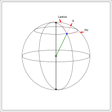
The potential from a zonal term is rotational symmetric around the polar axis of the Earth and corresponding force is entirely in a longitudial plane with one component $F_{r}\ {\hat {r}}\,$ in the radial direction and one component $F_{\lambda }\ {\hat {\lambda }}\,$ with the unit vector ${\hat {\lambda }}\,$ orthogonal to the radial direction towards north. These directions ${\hat {r}}\,$ and ${\hat {\lambda }}\,$ are illustrated in Figure 1.

Figure 1: The unit vectors

{\hat {\phi }}\ ,\ {\hat {\lambda }}\ ,\ {\hat {r}}

In the article Geopotential model it is shown that these force components caused by the $J_{3}\,$ term are

${\begin{aligned}&F_{r}=J_{3}\ {\frac {1}{r^{5}}}\ 2\ \sin \lambda \ \left(5\sin ^{2}\lambda \ -\ 3\right)\\&F_{\lambda }=-J_{3}\ {\frac {1}{r^{5}}}\ {\frac {3}{2}}\ \cos \lambda \ \left(5\ \sin ^{2}\lambda \ -1\right)\end{aligned}}$

(11)

To be able to apply relations derived in the article Orbital perturbation analysis (spacecraft) the force component $F_{\lambda }\ {\hat {\lambda }}\,$ must be split into two orthogonal components $F_{t}\ {\hat {t}}$ and $F_{z}\ {\hat {z}}$ as illustrated in figure 2

Figure 2: The unit vector

{\hat {t}}\,

orthogonal to

{\hat {r}}\,

in the direction of motion and the orbital pole

{\hat {z}}\,

. The force component

F_{\lambda }

is marked as "F"

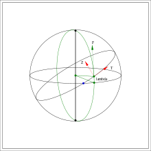
Let ${\hat {a}}\ ,\ {\hat {b}}\ ,\ {\hat {n}}\,$ make up a rectangular coordinate system with origin in the center of the Earth (in the center of the Reference ellipsoid) such that ${\hat {n}}\,$ points in the direction north and such that ${\hat {a}}\ ,\ {\hat {b}}\,$ are in the equatorial plane of the Earth with ${\hat {a}}\,$ pointing towards the ascending node, i.e. towards the blue point of Figure 2.

The components of the unit vectors

{\hat {r}}\ ,\ {\hat {t}}\ ,\ {\hat {z}}\,

making up the local coordinate system (of which ${\hat {t}}\ ,\ {\hat {z}},$ are illustrated in figure 2), and expressing their relation with ${\hat {a}}\ ,\ {\hat {b}}\ ,\ {\hat {n}}\,$ , are as follows:

r_{a}=\cos u\,

r_{b}=\cos i\ \sin u\,

r_{n}=\sin i\ \sin u\,

t_{a}=-\sin u\,

t_{b}=\cos i\ \cos u\,

t_{n}=\sin i\ \cos u\,

z_{a}=0\,

z_{b}=-\sin i\,

z_{n}=\cos i\,

where $u\,$ is the polar argument of ${\hat {r}}\,$ relative the orthogonal unit vectors ${\hat {g}}={\hat {a}}\,$ and ${\hat {h}}=\cos i\ {\hat {b}}\ +\ \sin i\ {\hat {n}}\,$ in the orbital plane

Firstly

\sin \lambda =\ r_{n}\ =\ \sin i\ \sin u\,

where $\lambda \,$ is the angle between the equator plane and ${\hat {r}}\,$ (between the green points of figure 2) and from equation (12) of the article Geopotential model one therefore obtains

$F_{r}=J_{3}\ {\frac {1}{r^{5}}}\ 2\ \sin i\ \sin u\,\ \left(5\sin ^{2}i\ \sin ^{2}u\ -\ 3\right)$

(12)

Secondly the projection of direction north, ${\hat {n}}\,$ , on the plane spanned by ${\hat {t}}\ ,\ {\hat {z}},$ is

\sin i\ \cos u\ {\hat {t}}\ +\ \cos i\ {\hat {z}}\,

and this projection is

\cos \lambda \ {\hat {\lambda }}\,

where ${\hat {\lambda }}\,$ is the unit vector ${\hat {\lambda }}$ orthogonal to the radial direction towards north illustrated in figure 1.

From equation (11) we see that

F_{\lambda }\ {\hat {\lambda }}\ =-J_{3}\ {\frac {1}{r^{5}}}\ {\frac {3}{2}}\ \left(5\ \sin ^{2}\lambda \ -1\right)\ \cos \lambda \ {\hat {\lambda }}\ =\ -J_{3}\ {\frac {1}{r^{5}}}\ {\frac {3}{2}}\ \left(5\ \sin ^{2}\lambda \ -1\right)\ (\sin i\ \cos u\ {\hat {t}}\ +\ \cos i\ {\hat {z}})\,

and therefore:

$F_{t}=\ -J_{3}\ {\frac {1}{r^{5}}}\ {\frac {3}{2}}\ \left(5\ \sin ^{2}i\ \sin ^{2}u\ -1\right)\ \sin i\ \cos u$

(13)

$F_{z}=\ -J_{3}\ {\frac {1}{r^{5}}}\ {\frac {3}{2}}\ \left(5\ \sin ^{2}i\ \sin ^{2}u\ -1\right)\ \cos i$

(14)

In the article Orbital perturbation analysis (spacecraft) it is further shown that the secular perturbation of the orbital pole ${\hat {z}}\,$ is

$\Delta {\hat {z}}\ =\ {\frac {1}{\mu p}}\left[{\hat {g}}\int \limits _{{0}}^{{2\pi }}F_{z}r^{3}\cos u\ du+\ {\hat {h}}\int \limits _{{0}}^{{2\pi }}F_{z}r^{3}\sin u\ du\right]\quad \times \ {\hat {z}}$

(15)

Introducing the expression for $F_{z}\,$ of (14) in (15) one gets

${\begin{aligned}&\Delta {\hat {z}}\ =-{\frac {J_{3}}{\mu \ p^{3}}}\ {\frac {3}{2}}\ \cos i\ \cdot \\&\left[{\hat {g}}\int \limits _{{0}}^{{2\pi }}{\left({\frac {p}{r}}\right)}^{2}\left(5\ \sin ^{2}i\ \sin ^{2}u\ -1\right)\cos u\ du\ +{\hat {h}}\int \limits _{{0}}^{{2\pi }}{\left({\frac {p}{r}}\right)}^{2}\left(5\ \sin ^{2}i\ \sin ^{2}u\ -1\right)\sin u\ du\right]\quad \times \ {\hat {z}}\end{aligned}}$

(16)

The fraction ${\frac {p}{r}}\,$ is

{\frac {p}{r}}\ =\ 1+e\cdot \cos \theta \ =\ 1+e_{g}\cdot \cos u+e_{h}\cdot \sin u

where

e_{g}=\ e\ \cos \omega

e_{h}=\ e\ \sin \omega

are the components of the eccentricity vector in the ${\hat {g}}\ ,\ {\hat {h}}\,$ coordinate system.

As all integrals of type

\int \limits _{{0}}^{{2\pi }}\cos ^{m}u\ \sin ^{n}u\ du\,

are zero if not both $n\,$ and $m\,$ are even, we see that

${\begin{aligned}\int \limits _{{0}}^{{2\pi }}{\left({\frac {p}{r}}\right)}^{2}\left(5\ \sin ^{2}i\ \sin ^{2}u\ -1\right)\cos u\ du&=\ 2\ e_{g}\ \left(5\ \sin ^{2}i\ \int \limits _{{0}}^{{2\pi }}\sin ^{2}u\cos ^{2}u\ du\ -\int \limits _{{0}}^{{2\pi }}\cos ^{2}u\ du\right)\\&=\ 2\pi \ e_{g}\ ({\frac {5}{4}}\sin ^{2}i-1)\end{aligned}}$

(17)

and

${\begin{aligned}\int \limits _{{0}}^{{2\pi }}{\left({\frac {p}{r}}\right)}^{2}\left(5\ \sin ^{2}i\ \sin ^{2}u\ -1\right)\sin u\ du&=\ 2\ e_{h}\ \left(5\ \sin ^{2}i\ \int \limits _{{0}}^{{2\pi }}\sin ^{4}u\ du\ -\int \limits _{{0}}^{{2\pi }}\sin ^{2}u\ du\right)\\&=\ 2\pi \ e_{h}\ ({\frac {15}{4}}\sin ^{2}i-1)\end{aligned}}$

(18)

It follows that

${\begin{aligned}\Delta {\hat {z}}\ &=\ 2\pi \ {\frac {J_{3}}{\mu \ p^{3}}}\ {\frac {3}{2}}\ \cos i\ \left[e_{g}\ (1-{\frac {5}{4}}\sin ^{2}i)\ {\hat {g}}+\ e_{h}\ (1-{\frac {15}{4}}\sin ^{2}i)\ {\hat {h}}\right]\quad \times \ {\hat {z}}\\&=\ 2\pi \ {\frac {J_{3}}{\mu \ p^{3}}}\ {\frac {3}{2}}\ \cos i\ \left[\ e_{h}\ (1-{\frac {15}{4}}\sin ^{2}i)\ {\hat {g}}\ -e_{g}\ (1-{\frac {5}{4}}\sin ^{2}i)\ {\hat {h}}\right]\end{aligned}}$

(19)

where

{\hat {g}}\,

and

{\hat {h}}\,

are the base vectors of the rectangular coordinate system in the plane of the reference Kepler orbit with

{\hat {g}}\,

in the equatorial plane towards the ascending node and

u\,

is the polar argument relative this equatorial coordinate system

f_{z}\,

is the force component (per unit mass) in the direction of the orbit pole

{\hat {z}}\,

In the article Orbital perturbation analysis (spacecraft) it is shown that the secular perturbation of the eccentricity vector is

$\Delta {\bar {e}}\ ={\frac {1}{\mu }}\ \int \limits _{{0}}^{{2\pi }}\left(-{\hat {t}}\ f_{r}\ +\ \left(2\ {\hat {r}}-{\frac {V_{r}}{V_{t}}}\ {\hat {t}}\right)\ f_{t}\right)\ r^{2}\ du$

(20)

where

${\hat {r}}\ ,{\hat {t}}\,$ is the usual local coordinate system with unit vector ${\hat {r}}\,$ directed away from the Earth
$V_{r}={\sqrt {{\frac {\mu }{p}}}}\cdot e\cdot \sin \theta$ - the velocity component in direction ${\hat {r}}\,$
$V_{t}={\sqrt {{\frac {\mu }{p}}}}\cdot (1+e\cdot \cos \theta )$ - the velocity component in direction ${\hat {t}}\,$

Introducing the expression for $F_{r}\ ,\ F_{t}\,$ of (12) and (13) in (20) one gets

${\begin{aligned}&\Delta {\bar {e}}\ ={\frac {J_{3}}{\mu \ p^{3}}}\ \sin i\ \cdot \\&\int \limits _{{0}}^{{2\pi }}\left(-{\hat {t}}\ {\left({\frac {p}{r}}\right)}^{3}\ 2\ \sin u\,\ \left(5\sin ^{2}i\ \sin ^{2}u\ -\ 3\right)\ -\ \left(2\ {\hat {r}}-{\frac {V_{r}}{V_{t}}}\ {\hat {t}}\right)\ {\left({\frac {p}{r}}\right)}^{3}\ {\frac {3}{2}}\ \left(5\ \sin ^{2}i\ \sin ^{2}u\ -1\right)\ \cos u\right)du\end{aligned}}$

(21)

Using that

{\frac {V_{r}}{V_{t}}}={\frac {e_{g}\cdot \sin u\ -\ e_{h}\cdot \cos u}{{\frac {p}{r}}}}

the integral above can be split in 8 terms:

${\begin{aligned}&\int \limits _{{0}}^{{2\pi }}\left(-{\hat {t}}\ {\left({\frac {p}{r}}\right)}^{3}\ 2\ \sin u\,\ \left(5\sin ^{2}i\ \sin ^{2}u\ -\ 3\right)\ -\ \left(2\ {\hat {r}}-{\frac {V_{r}}{V_{t}}}\ {\hat {t}}\right)\ {\left({\frac {p}{r}}\right)}^{3}\ {\frac {3}{2}}\ \left(5\ \sin ^{2}i\ \sin ^{2}u\ -1\right)\ \cos u\right)\ du\ =\\&-10\sin ^{2}i\ \int \limits _{{0}}^{{2\pi }}{\hat {t}}\ {\left({\frac {p}{r}}\right)}^{3}\ \sin ^{3}u\ du\\&+6\ \int \limits _{{0}}^{{2\pi }}{\hat {t}}\ {\left({\frac {p}{r}}\right)}^{3}\ \sin u\ du\\&-15\ \sin ^{2}i\int \limits _{{0}}^{{2\pi }}{\hat {r}}\ {\left({\frac {p}{r}}\right)}^{3}\ \sin ^{2}u\ \cos u\ du\\&+3\ \int \limits _{{0}}^{{2\pi }}{\hat {r}}\ {\left({\frac {p}{r}}\right)}^{3}\ \cos u\ du\\&+{\frac {15}{2}}\sin ^{2}i\ e_{g}\int \limits _{{0}}^{{2\pi }}{\hat {t}}\ {\left({\frac {p}{r}}\right)}^{2}\ \ \ \sin ^{3}u\ \cos u\ du\\&-{\frac {15}{2}}\sin ^{2}i\ e_{h}\ \int \limits _{{0}}^{{2\pi }}{\hat {t}}\ {\left({\frac {p}{r}}\right)}^{2}\ \ \ \sin ^{2}u\ \cos ^{2}u\ du\\&-{\frac {3}{2}}\ e_{g}\ \int \limits _{{0}}^{{2\pi }}\ {\hat {t}}\ {\left({\frac {p}{r}}\right)}^{2}\ \ \sin u\ \cos u\ du\\&+{\frac {3}{2}}\ e_{h}\ \int \limits _{{0}}^{{2\pi }}{\hat {t}}\ {\left({\frac {p}{r}}\right)}^{2}\ \ \cos ^{2}u\ du\end{aligned}}$

(22)

Given that

{\hat {r}}=\cos u\ {\hat {g}}\ +\ \sin u\ {\hat {h}}

{\hat {t}}=-\sin u\ {\hat {g}}\ +\ \cos u\ {\hat {h}}

we obtain

{\frac {p}{r}}\ =\ 1+e\cdot \cos \theta \ =\ 1+e_{g}\cdot \cos u+e_{h}\cdot \sin u

and that all integrals of type

\int \limits _{{0}}^{{2\pi }}\cos ^{m}u\ \sin ^{n}u\ du\,

are zero if not both $n\,$ and $m\,$ are even:

Term 1

${\begin{aligned}&\int \limits _{{0}}^{{2\pi }}{\hat {t}}\ {\left({\frac {p}{r}}\right)}^{3}\ \sin ^{3}u\ du\ =-{\hat {g}}\ \int \limits _{{0}}^{{2\pi }}\ {\left({\frac {p}{r}}\right)}^{3}\ \sin ^{4}u\ du\ +{\hat {h}}\int \limits _{{0}}^{{2\pi }}\ {\left({\frac {p}{r}}\right)}^{3}\ \sin ^{3}u\ \cos u\ du\ =\\&-{\hat {g}}\ \left(\int \limits _{{0}}^{{2\pi }}\ \sin ^{4}u\ du\ +\ 3\ {e_{g}}^{2}\ \int \limits _{{0}}^{{2\pi }}\ \cos ^{2}u\ \sin ^{4}u\ du\ \ +\ 3\ {e_{h}}^{2}\ \int \limits _{{0}}^{{2\pi }}\ \sin ^{6}u\ du\ \right)\\&+{\hat {h}}\ 6\ e_{g}\ e_{h}\ \int \limits _{{0}}^{{2\pi }}\ \cos ^{2}u\ \sin ^{4}u\ du=\\&-{\hat {g}}\ \left(2\pi \left({\frac {3}{8}}\ +\ {\frac {3}{16}}\ {e_{g}}^{2}\ +\ {\frac {15}{16}}\ {e_{h}}^{2}\right)\right)+{\hat {h}}\ \left(2\pi \left({\frac {3}{8}}\ e_{g}\ e_{h}\right)\right)\end{aligned}}$

(23)

Term 2

${\begin{aligned}&\int \limits _{{0}}^{{2\pi }}{\hat {t}}\ {\left({\frac {p}{r}}\right)}^{3}\ \sin u\ du\ =-{\hat {g}}\ \int \limits _{{0}}^{{2\pi }}\ {\left({\frac {p}{r}}\right)}^{3}\ \sin ^{2}u\ du\ +{\hat {h}}\int \limits _{{0}}^{{2\pi }}\ {\left({\frac {p}{r}}\right)}^{3}\ \sin u\ \cos u\ du\ =\\&-{\hat {g}}\ \left(\int \limits _{{0}}^{{2\pi }}\ \sin ^{2}u\ du\ +\ 3\ {e_{g}}^{2}\ \int \limits _{{0}}^{{2\pi }}\ \cos ^{2}u\ \sin ^{2}u\ du\ \ +\ 3\ {e_{h}}^{2}\ \int \limits _{{0}}^{{2\pi }}\ \sin ^{6}u\ du\ \right)\\&+{\hat {h}}\ 6\ e_{g}\ e_{h}\ \int \limits _{{0}}^{{2\pi }}\ \cos ^{2}u\ \sin ^{2}u\ du=\\&-{\hat {g}}\ \left(2\pi \left({\frac {1}{2}}\ +\ {\frac {3}{8}}\ {e_{g}}^{2}\ +\ {\frac {9}{8}}\ {e_{h}}^{2}\right)\right)+{\hat {h}}\ \left(2\pi \left({\frac {3}{4}}\ e_{g}\ e_{h}\right)\right)\end{aligned}}$

(24)

Term 3

${\begin{aligned}&\int \limits _{{0}}^{{2\pi }}{\hat {r}}\ {\left({\frac {p}{r}}\right)}^{3}\ \sin ^{2}u\ \cos u\ du\ ={\hat {g}}\ \int \limits _{{0}}^{{2\pi }}\ {\left({\frac {p}{r}}\right)}^{3}\ \sin ^{2}u\cos ^{2}u\ du\ +{\hat {h}}\int \limits _{{0}}^{{2\pi }}\ {\left({\frac {p}{r}}\right)}^{3}\ \sin ^{3}u\ \cos u\ du\ =\\&{\hat {g}}\ \left(\int \limits _{{0}}^{{2\pi }}\ \sin ^{2}u\cos ^{2}u\ du\ +\ 3\ {e_{g}}^{2}\ \int \limits _{{0}}^{{2\pi }}\ \cos ^{4}u\ \sin ^{2}u\ du\ \ +\ 3\ {e_{h}}^{2}\ \int \limits _{{0}}^{{2\pi }}\ \sin ^{4}u\ \cos ^{2}u\ du\ \right)\\&+{\hat {h}}\ 6\ e_{g}\ e_{h}\ \int \limits _{{0}}^{{2\pi }}\ \cos ^{2}u\ \sin ^{4}u\ du=\\&{\hat {g}}\ \left(2\pi \left({\frac {1}{8}}\ +\ {\frac {3}{16}}\ {e_{g}}^{2}\ +\ {\frac {3}{16}}\ {e_{h}}^{2}\right)\right)+{\hat {h}}\ \left(2\pi \left({\frac {3}{8}}\ e_{g}\ e_{h}\right)\right)\end{aligned}}$

(25)

Term 4

${\begin{aligned}&\int \limits _{{0}}^{{2\pi }}{\hat {r}}\ {\left({\frac {p}{r}}\right)}^{3}\ \cos u\ du\ ={\hat {g}}\ \int \limits _{{0}}^{{2\pi }}\ {\left({\frac {p}{r}}\right)}^{3}\ \cos ^{2}u\ du\ +{\hat {h}}\int \limits _{{0}}^{{2\pi }}\ {\left({\frac {p}{r}}\right)}^{3}\ \sin u\ \cos u\ du\ =\\&{\hat {g}}\ \left(\int \limits _{{0}}^{{2\pi }}\cos ^{2}u\ du\ +\ 3\ {e_{g}}^{2}\ \int \limits _{{0}}^{{2\pi }}\ \cos ^{4}u\ du\ \ +\ 3\ {e_{h}}^{2}\ \int \limits _{{0}}^{{2\pi }}\ \sin ^{2}u\ \cos ^{2}u\ du\ \right)\\&+{\hat {h}}\ 6\ e_{g}\ e_{h}\ \int \limits _{{0}}^{{2\pi }}\ \cos ^{2}u\ \sin ^{2}u\ du=\\&{\hat {g}}\ \left(2\pi \left({\frac {1}{2}}\ +\ {\frac {9}{8}}\ {e_{g}}^{2}\ +\ {\frac {3}{8}}\ {e_{h}}^{2}\right)\right)+{\hat {h}}\ \left(2\pi \left({\frac {3}{4}}\ e_{g}\ e_{h}\right)\right)\end{aligned}}$

(26)

Term 5

${\begin{aligned}&\int \limits _{{0}}^{{2\pi }}{\hat {t}}\ {\left({\frac {p}{r}}\right)}^{2}\ \sin ^{3}u\ \cos u\ du\ =-{\hat {g}}\ \int \limits _{{0}}^{{2\pi }}\ {\left({\frac {p}{r}}\right)}^{2}\ \sin ^{4}u\ \cos u\ du\ +{\hat {h}}\int \limits _{{0}}^{{2\pi }}\ {\left({\frac {p}{r}}\right)}^{2}\ \sin ^{3}u\ \cos ^{2}u\ du\ =\\&-{\hat {g}}\ 2\ e_{g}\ \int \limits _{{0}}^{{2\pi }}\ \sin ^{4}u\ \cos ^{2}u\ du+{\hat {h}}\ 2\ e_{h}\ \int \limits _{{0}}^{{2\pi }}\ \sin ^{4}u\ \cos ^{2}u\ du=-{\hat {g}}\ \left(2\pi {\frac {1}{8}}\ e_{g}\right)+{\hat {h}}\ \left(2\pi {\frac {1}{8}}\ e_{h}\right)\end{aligned}}$

(27)

Term 6

${\begin{aligned}&\int \limits _{{0}}^{{2\pi }}{\hat {t}}\ {\left({\frac {p}{r}}\right)}^{2}\ \sin ^{2}u\ \cos ^{2}u\ du\ =-{\hat {g}}\ \int \limits _{{0}}^{{2\pi }}\ {\left({\frac {p}{r}}\right)}^{2}\ \sin ^{3}u\ \cos ^{2}u\ du\ +{\hat {h}}\int \limits _{{0}}^{{2\pi }}\ {\left({\frac {p}{r}}\right)}^{2}\ \sin ^{2}u\ \cos ^{3}u\ du\ =\\&-{\hat {g}}\ 2\ e_{h}\ \int \limits _{{0}}^{{2\pi }}\ \sin ^{4}u\ \cos ^{2}u\ du+{\hat {h}}\ 2\ e_{g}\ \int \limits _{{0}}^{{2\pi }}\ \sin ^{2}u\ \cos ^{4}u\ du=-{\hat {g}}\ \left(2\pi {\frac {1}{8}}\ e_{h}\right)+{\hat {h}}\ \left(2\pi {\frac {1}{8}}\ e_{g}\right)\end{aligned}}$

(28)

Term 7

${\begin{aligned}&\int \limits _{{0}}^{{2\pi }}{\hat {t}}\ {\left({\frac {p}{r}}\right)}^{2}\ \sin u\ \cos u\ du\ =-{\hat {g}}\ \int \limits _{{0}}^{{2\pi }}\ {\left({\frac {p}{r}}\right)}^{2}\ \sin ^{2}u\ \cos u\ du\ +{\hat {h}}\int \limits _{{0}}^{{2\pi }}\ {\left({\frac {p}{r}}\right)}^{2}\ \sin u\ \cos ^{2}u\ du\ =\\&-{\hat {g}}\ 2\ e_{g}\ \int \limits _{{0}}^{{2\pi }}\ \sin ^{2}u\ \cos ^{2}u\ du+{\hat {h}}\ 2\ e_{h}\ \int \limits _{{0}}^{{2\pi }}\ \sin ^{2}u\ \cos ^{2}u\ du=-{\hat {g}}\ \left(2\pi {\frac {1}{4}}\ e_{g}\right)+{\hat {h}}\ \left(2\pi {\frac {1}{4}}\ e_{h}\right)\end{aligned}}$

(29)

Term 8

${\begin{aligned}&\int \limits _{{0}}^{{2\pi }}{\hat {t}}\ {\left({\frac {p}{r}}\right)}^{2}\ \cos ^{2}u\ du\ =-{\hat {g}}\ \int \limits _{{0}}^{{2\pi }}\ {\left({\frac {p}{r}}\right)}^{2}\ \sin u\ \cos ^{2}u\ du\ +{\hat {h}}\int \limits _{{0}}^{{2\pi }}\ {\left({\frac {p}{r}}\right)}^{2}\ \cos ^{3}u\ du\ =\\&-{\hat {g}}\ 2\ e_{h}\ \int \limits _{{0}}^{{2\pi }}\ \sin ^{2}u\ \cos ^{2}u\ du+{\hat {h}}\ 2\ e_{g}\ \int \limits _{{0}}^{{2\pi }}\ \cos ^{4}u\ du=-{\hat {g}}\ \left(2\pi {\frac {1}{4}}\ e_{h}\right)+{\hat {h}}\ \left(2\pi {\frac {3}{4}}\ e_{g}\right)\end{aligned}}$

(30)

As

${\begin{aligned}&-10\sin ^{2}i\ \left(-{\hat {g}}\ \left({\frac {3}{8}}\ +\ {\frac {3}{16}}\ {e_{g}}^{2}\ +\ {\frac {15}{16}}\ {e_{h}}^{2}\right)+{\hat {h}}\ \left({\frac {3}{8}}\ e_{g}\ e_{h}\right)\right)\\&+6\ \left(-{\hat {g}}\ \left({\frac {1}{2}}\ +\ {\frac {3}{8}}\ {e_{g}}^{2}\ +\ {\frac {9}{8}}\ {e_{h}}^{2}\right)+{\hat {h}}\ \left({\frac {3}{4}}\ e_{g}\ e_{h}\right)\right)\\&-15\sin ^{2}i\ \left({\hat {g}}\ \left({\frac {1}{8}}\ +\ {\frac {3}{16}}\ {e_{g}}^{2}\ +\ {\frac {3}{16}}\ {e_{h}}^{2}\right)+{\hat {h}}\ \left({\frac {3}{8}}\ e_{g}\ e_{h}\right)\right)\\&+3\left({\hat {g}}\ \left({\frac {1}{2}}\ +\ {\frac {9}{8}}\ {e_{g}}^{2}\ +\ {\frac {3}{8}}\ {e_{h}}^{2}\right)+{\hat {h}}\ \left({\frac {3}{4}}\ e_{g}\ e_{h}\right)\right)\\&+{\frac {15}{2}}\sin ^{2}i\ e_{g}\ \left(-{\hat {g}}\ \left({\frac {1}{8}}\ e_{g}\right)+{\hat {h}}\ \left({\frac {1}{8}}\ e_{h}\right)\right)\\&-{\frac {15}{2}}\sin ^{2}i\ e_{h}\ \left(-{\hat {g}}\ \left({\frac {1}{8}}\ e_{h}\right)+{\hat {h}}\ \left({\frac {1}{8}}\ e_{g}\right)\right)\\&-{\frac {3}{2}}\ e_{g}\ \left(-{\hat {g}}\ \left({\frac {1}{4}}\ e_{g}\right)+{\hat {h}}\ \left({\frac {1}{4}}\ e_{h}\right)\right)\\&+{\frac {3}{2}}\ e_{h}\ \left(-{\hat {g}}\ \left({\frac {1}{4}}\ e_{h}\right)+{\hat {h}}\ \left({\frac {3}{4}}\ e_{g}\right)\right)=\\&{\frac {3}{2}}\ \left({\frac {5}{4}}\ \sin ^{2}i\ -\ 1\right)\left((1-{e_{g}}^{2}\ +\ 4\ {e_{h}}^{2}){\hat {g}}\ -\ 5\ e_{g}\ e_{h}\ {\hat {h}}\right)\end{aligned}}$

(31)

It follows that

${\begin{aligned}&\Delta {\bar {e}}\ ={\frac {J_{3}}{\mu \ p^{3}}}\ \sin i\ \cdot \\&\int \limits _{{0}}^{{2\pi }}\left(-{\hat {t}}\ {\left({\frac {p}{r}}\right)}^{3}\ 2\ \sin u\,\ \left(5\sin ^{2}i\ \sin ^{2}u\ -\ 3\right)\ -\ \left(2\ {\hat {r}}-{\frac {V_{r}}{V_{t}}}\ {\hat {t}}\right)\ {\left({\frac {p}{r}}\right)}^{3}\ {\frac {3}{2}}\ \left(5\ \sin ^{2}i\ \sin ^{2}u\ -1\right)\ \cos u\right)du=\\&2\pi \ {\frac {J_{3}}{\mu \ p^{3}}}\ \sin i\ {\frac {3}{2}}\ \left({\frac {5}{4}}\ \sin ^{2}i\ -\ 1\right)\left((1-{e_{g}}^{2}\ +\ 4\ {e_{h}}^{2}){\hat {g}}\ -\ 5\ e_{g}\ e_{h}\ {\hat {h}}\right)\end{aligned}}$

(32)

References

↑ Eagle, C. David. "Frozen Orbit Design" (PDF). Orbital Mechanics with Numerit. Archived from the original (PDF) on 21 November 2011. Retrieved 5 April 2012.
↑ Chobotov, Vladimir A. (2002). Orbital Mechanics (3rd ed.). American Institute of Aeronautics and Astronautics. p. 221.
↑ Frozen Orbits About the Moon. 2003
↑ Bell, Trudy E. (November 6, 2006). Phillips, Tony, ed. "Bizarre Lunar Orbits". Science@NASA. NASA. Retrieved 2017-09-08.
↑ Dirk Brouwer: "Solution of the Problem of the Artificial Satellite Without Drag", Astronomical Journal, 64 (1959)
↑ Mats Rosengren (1989). "Improved technique for Passive Eccentricity Control (AAS 89-155)". Advances in the Astronautical Sciences. 69. AAS/NASA. Bibcode:1989ommd.proc...49R.

Frozen orbit

Background and motivation

Lunar frozen orbits

Classical theory

Modern theory

Derivation of the closed form expressions for the J3 perturbation

References

Further reading