Boundary tracing
Boundary tracing (also known as contour tracing) of a binary digital region can be thought of as a segmentation technique that identifies the boundary pixels of the digital region. Boundary tracing is an important first step in the analysis of that region.
Algorithms
Algorithms used for boundary tracing:[1]
- Square Tracing algorithm[2]
- Moore-Neighbor Tracing algorithm
- Radial Sweep [3]
- Theo Pavlidis’ algorithm [4]
- an algorithm created by Dr Kovalevsky using modulo division and simple pixel lookups
- A generic approach using vector algebra for tracing of a boundary can be found at.[5]
- An extension of boundary tracing for segmentation of traced boundary into open and closed sub-section is described at.[6]
Dr Kovalevsky Algorithm
With an abstract cell complex representation of a digital image, the boundary point coordinates may be extracted from that digital image by following an algorithm created by Dr Kovalevsky using modulo division and simple pixel lookups.
This algorithm:
- assumes a single connected region within the binary image
- begins with an exhaustive search to locate the first foreground pixel by iterating over the columns and rows of the image.

// 2D Point data structure
struct Point
{
    int x; // col
    int y; // row

    P(int a , int b)
    {
        x = a;
        y = b;
    };
};

// Example Image Data
const int width  = 6;
const int height = 10;
int[height][width] image = { { 0 , 0 , 0 , 0 , 0 , 0 } ,
                             { 0 , 0 , 1 , 1 , 1 , 1 } ,
                             { 0 , 0 , 1 , 1 , 1 , 1 } ,
                             { 0 , 1 , 1 , 1 , 1 , 1 } ,
                             { 1 , 1 , 1 , 1 , 1 , 0 } ,
                             { 1 , 1 , 1 , 1 , 1 , 0 } ,
                             { 0 , 0 , 1 , 1 , 1 , 0 } ,
                             { 0 , 0 , 1 , 1 , 1 , 0 } ,
                             { 0 , 0 , 1 , 1 , 1 , 0 } ,
                             { 0 , 0 , 0 , 0 , 0 , 0 } };

// Exhaustive row-major order search for first foreground pixel
Point startPoint;
for ( int row = 0 ; row < height ; row++ )
{
    for ( int col = 0 ; col < width ; col++ )
    {
        if ( image[row][col] == 1 )
        {
           startPoint.x = col;
           startPoint.y = row;
           return;
        }
    }
}
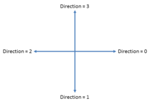
Once that pixel is located the algorithm may begin by tracing the cracks of the region in a counterclockwise fashion following one of four possible directions at each step. These directions are represented by a crack code sequence: 0 (East), 1 (South), 2 (West), 3 (North)
See also
References
- ↑ Contour Tracing Algorithms
- ↑ Abeer George Ghuneim: square tracing algorithm
- ↑ Abeer George Ghuneim: The Radial Sweep algorithm
- ↑ Abeer George Ghuneim: Theo Pavlidis' Algorithm
- ↑ Vector Algebra Based Tracing of External and Internal Boundary of an Object in Binary Images, Journal of Advances in Engineering Science Volume 3 Issue 1, January - June 2010, PP 57-70
- ↑ Graph theory based segmentation of traced boundary into open and closed sub-sections, Computer Vision and Image Understanding, Volume 115, Issue 11, November 2011, Pages 1552–1558