Bond graph

A simple mass–spring–damper system, and its equivalent bond-graph form

A bond graph is a graphical representation of a physical dynamic system. It allows the conversion of the system into a state-space representation. It is similar to a block diagram or signal-flow graph, with the major difference that the arcs in bond graphs represent bi-directional exchange of physical energy, while those in block diagrams and signal-flow graphs represent uni-directional flow of information. Bond graphs are multi-energy domain (e.g. mechanical, electrical, hydraulic, etc) and domain neutral. This means a bond graph can incorporate multiple domains seamlessly.

The bond graph is composed of the "bonds" which link together "single port", "double-port" and "multi-port" elements (see below for details). Each bond represents the instantaneous flow of energy (dE/dt) or power. The flow in each bond is denoted by a pair of variables called power variables, whose product is the instantaneous power of the bond. The power variables are broken into two parts: flow and effort. For example, for the bond of an electrical system, the flow is the current, while the effort is the voltage. By multiplying current and voltage in this example you can get the instantaneous power of the bond.

A bond has two other features described briefly here, and discussed in more detail below. One is the "half-arrow" sign convention. This defines the assumed direction of positive energy flow. As with electrical circuit diagrams and free-body diagrams, the choice of positive direction is arbitrary, with the caveat that the analyst must be consistent throughout with the chosen definition. The other feature is the "causality". This is a vertical bar placed on only one end of the bond. It is not arbitrary. As described below, there are rules for assigning the proper causality to a given port, and rules for the precedence among ports. Causality explains the mathematical relationship between effort and flow. The positions of the causalities show which of the power variables are dependent and which are independent.

If the dynamics of the physical system to be modeled operate on widely varying time scales, fast continuous-time behaviors can be modeled as instantaneous phenomena by using a hybrid bond graph. Bond graphs were invented by Henry Paynter.^[1]

Tetrahedron of state

Tetrahedron of state

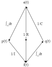
The tetrahedron of state is a tetrahedron that graphically shows the conversion between effort and flow. The image to the right shows the tetrahedron in its generalized form. The tetrahedron can be modified depending on the energy domain. The table below shows the variables and constants of the tetrahedron of state in common energy domains.

Energy Domain^[2]^{[Note 1]}		$f(t)$	$e(t)$	$q(t)$	$p(t)$	$R$	$I$	$C$
Generalized	Name	Generalized flow	Generalized effort	Generalized displacement	Generalized momentum	Resistance	Inertance	Compliance
Generalized	Symbol	$f(t)$	$e(t)$	$q(t)$	$p(t)$	$R$	$I$	$C$
Linear mechanical	Name	Velocity	Force	Displacement	Linear momentum	Damping constant	Mass	Inverse of the spring constant
	Symbol	$v(t)$	$F(t)$	$x(t)$	$p(t)$	$b$	$m$	${\frac {1}{k}}$
	Units	$m/s$	$N$	$m$	$N\cdot s$	$N\cdot s/m$	$kg$	$m/N$
Angular mechanical	Name	Angular velocity	Torque	Angular displacement	Angular momentum	Angular damping	Mass moment of inertia	Inverse of the angular spring constant
	Symbol	$\omega (t)$	$T(t)$	$\theta (t)$	$p_{\tau }(t)$	$B$	$J$	${\frac {1}{k_{\tau }}}$
	Units	$rad/s$	$N\cdot m$	$rad$	$N\cdot m\cdot s$	$rad/(N\cdot m\cdot s)$	$kg\cdot m^{2}$	$1/(N\cdot m)$
Electromagnetic	Name	Current	Voltage	Charge	Flux linkage	Resistance	Inductance	Capacitance
	Symbol	$i(t)$	$V(t)$	$q(t)$	$\lambda (t)$	$R$	$L$	$C$
	Units	$A$	$V$	$C$	$V\cdot s$	$\Omega$	$H$	$F$
Hydraulic/ pneumatic	Name	Volume flow rate	Pressure	Volume	Fluid momentum	Fluid resistance	Fluid inductance	Storage
	Symbol	$\varphi (t)$	$P(t)$	$V(t)$	$p_{f}(t)$	$R_{f}$	$I_f$	$C_{f}$
	Units	$m^{3}/s$	$Pa$	$m^{3}$	$Pa\cdot s$	$Pa\cdot s/m^{3}$	$Pa\cdot s^{2}/m^{3}$	$m^{3}/Pa$

Using the tetrahedron of state, one can find a mathematical relationship between any variables on the tetrahedron. This is done by following the arrows around the diagram and multiplying any constants along the way. For example, if you wanted to find the relationship between generalized flow and generalized displacement, you would start at the f(t) and then integrate it to get q(t). More examples of equations can be seen below.

Relationship between generalized displacement and generalized flow.

$q(t)=\int f(t)\operatorname {d} \!t$

Relationship between generalized flow and generalized effort.

$f(t)={\frac {1}{R}}\cdot e(t)$

Relationship between generalized flow and generalized momentum.

$f(t)={\frac {1}{I}}\cdot p(t)$

Relationship between generalized momentum and generalized effort.

$p(t)=\int e(t)\operatorname {d} \!t$

Relationship between generalized flow and generalized involving the constant C.

$e(t)={\frac {1}{C}}\int f(t)\operatorname {d} \!t$

All of the mathematical relationships remain the same when switching energy domains, only the symbols change. This can be seen with the following examples.

Relationship between displacement and velocity.

$x(t)=\int v(t)\operatorname {d} \!t$

Relationship between current and voltage, this is also known as Ohm's law.

$i(t)={\frac {1}{R}}\cdot V(t)$

Relationship between force and displacement, also known as Hooke's law. It should be noted that the negative sign is dropped in this equation because the sign is factored into the way the arrow is pointing in the bond graph.

$F(t)=k\cdot x(t)$

Components

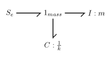
If an engine is connected to a wheel through a shaft, the power is being transmitted in the rotational mechanical domain, meaning the effort and the flow are torque (τ) and angular velocity (ω) respectively. A word bond graph is a first step towards a bond graph, in which words define the components. As a word bond graph, this system would look like:

{\text{engine}}\;\overset{\textstyle\tau}{\underset{\textstyle\omega}{-\!\!\!-\!\!\!-\!\!\!-\!\!\!-}}\;\text{wheel}

A half-arrow is used to provide a sign convention, so if the engine is doing work when τ and ω are positive, then the diagram would be drawn:

{\text{engine}}\;\overset{\textstyle\tau}{\underset{\textstyle\omega}{-\!\!\!-\!\!\!-\!\!\!\rightharpoondown}}\;\text{wheel}

This system can also be represented in a more general method. This involves changing from using the words, to symbols representing the same items. These symbols are based on the generalized form, as explained above. As the engine is applying a torque to the wheel, it will be represented as a source of effort for the system. The wheel can be presented by an impedance on the system. Further, the torque and angular velocity symbols are dropped and replaced with the generalized symbols for effort and flow. While not necessary in the example, it is common to number the bonds, to keep track of in equations. The simplified diagram can be seen below.

${S_{e}}\;{\overset {\textstyle e_{1}}{\underset {\textstyle f_{1}}{-\!\!\!-\!\!\!-\!\!\!\rightharpoondown }}}\;{\text{I}}$

Given that effort is always above the flow on the bond, it is also possible to drop the effort and flow symbols altogether, without losing any relevant information. However, the bond number should not be dropped. The example can be seen below.

${S_{e}}\;{\overset {\textstyle _{1}}{\underset {\textstyle }{-\!\!\!-\!\!\!-\!\!\!\rightharpoondown }}}\;{\text{I}}$

The bond number will be important later when converting from the bond graph to state-space equations.

Single-port elements

Single port elements are elements in a bond graph that can have only one port.

Sources and sinks

Sources are elements that represent the input for a system. They will either input effort or flow into a system. They are denoted by a capital "S" with either a lower case "e" or "f" for effort or flow respectively. Sources will always have the arrow pointing away from the element. An examples of sources include: motors (source of effort, torque), voltage sources (source of effort), and current sources (source of flow).

$S_{e}\;{\overset {\textstyle }{\underset {\textstyle }{-\!\!\!-\!\!\!-\!\!\!\rightharpoonup \!\!\!}}}\;\ J\qquad {\text{and}}\qquad S_{f}\;{\overset {\textstyle }{\underset {\textstyle }{-\!\!\!-\!\!\!-\!\!\!\rightharpoonup \!\!\!}}}\;\ J$

Sinks are elements that represent the output for a system. They are represented the same way as sources, but have the arrow pointing into the element instead of away from it.

$J\;{\overset {\textstyle }{\underset {\textstyle }{-\!\!\!-\!\!\!-\!\!\!\rightharpoonup \!\!\!}}}\;\ S_{e}\qquad {\text{and}}\qquad J\;{\overset {\textstyle }{\underset {\textstyle }{-\!\!\!-\!\!\!-\!\!\!\rightharpoonup \!\!\!}}}\;\ S_{f}$

Inertance

Inertance elements are denoted by a capital "I", and always have power flowing into them. Inertance elements are elements that store kinetic energy. Most commonly these are a mass for mechanical systems, and inductors for electrical systems.

$J\;{\overset {\textstyle }{\underset {\textstyle }{-\!\!\!-\!\!\!-\!\!\!\rightharpoonup \!\!\!}}}\;\ I$

Resistance

Resistance elements are denoted by a capital "R", and always have power flowing into them. Resistance elements are elements that dissipate energy. Most commonly these are a dampener, for mechanical systems, and resistors for electrical systems.

$J\;{\overset {\textstyle }{\underset {\textstyle }{-\!\!\!-\!\!\!-\!\!\!\rightharpoonup \!\!\!}}}\;\ R$

Capacitance

Capacitance elements are denoted by a capital "C", and always have power flowing into them. Capacitance elements are elements that store potential energy. Most commonly these are springs for mechanical systems, and capacitors for electrical systems.

$J\;{\overset {\textstyle }{\underset {\textstyle }{-\!\!\!-\!\!\!-\!\!\!\rightharpoonup \!\!\!}}}\;\ C$

Two-port elements

These elements have two ports. They are used to change the power between or within a system. When converting from one to the other, no power is lost during the transfer. The elements have a constant that will be given with it. The constant is called a transformer constant or gyrator constant depending on which element is being used. These constants will commonly be displayed as a ratio below the element.

Transformer

A transformer applies a relationship between flow in flow out, and effort in effort out. Examples include an ideal electrical transformer or a lever.

Denoted

${\begin{matrix}{\overset {\textstyle _{1}}{\underset {\textstyle }{\!\!\!-\!\!\!-\!\!\!-\!\!\!\rightharpoonup }}}\ \ \ TR\ \ {\overset {\textstyle _{2}}{\underset {\textstyle }{\!\!\!-\!\!\!-\!\!\!-\!\!\!\rightharpoonup }}}\ \\^{r:1}\end{matrix}}$

where the r denotes the modulus of the transformer. This means

f_{1}\cdot r=f_{2}

and

e_{2}\cdot r=e_{1}

Gyrator

A gyrator applies a relationship between flow in effort out, and effort in flow out. An example of a gyrator is a DC motor, which converts voltage (electrical effort) into Angular velocity (angular mechanical flow).

${\begin{matrix}{\overset {\textstyle _{1}}{\underset {\textstyle }{\!\!\!-\!\!\!-\!\!\!-\!\!\!\rightharpoonup }}}\ \ \ GY\ \ {\overset {\textstyle _{2}}{\underset {\textstyle }{\!\!\!-\!\!\!-\!\!\!-\!\!\!\rightharpoonup }}}\ \\^{g:1}\end{matrix}}$

meaning that

e_{2}=g\cdot f_{1}\,

and

e_{1}=g\cdot f_{2}.\,

Multi-port elements

Junctions, unlike the other elements can have any number of ports either in or out. Junctions split power across their ports. There are two distant junctions, the 0-junction and the 1-junction which differ only in the how effort and flow are carried across. It should be noted that the same junction in series can be combined, but different junctions in series cannot.

0-junctions

0-junctions behave such that all efforts values are equal across the bonds, but the sum of the flow values in equals the sum the flow values out.

$all\ e's\ are\ equal$

$\sum f_{in}=\sum f_{out}$

An example is shown below.

${\overset {\textstyle _{1}}{\underset {\textstyle }{-\!\!\!-\!\!\!-\!\!\!\rightharpoondown }}}{\stackrel {\textstyle {\stackrel {\textstyle _{2}}{\upharpoonright }}}{0}}{\overset {\textstyle _{3}}{\underset {\textstyle }{-\!\!\!-\!\!\!-\!\!\!\rightharpoondown }}}$

Resulting equations:

$e_{1}=e_{2}=e_{3}$

$f_{1}=f_{2}+f_{3}$

1-junctions

1-junctions behave opposite of 0-junctions. 1-junctions behave such that all flow values are equal across the bonds, but the sum of the effort values in equals the sum the effort values out.

$all\ f's\ are\ equal$

$\sum e_{in}=\sum e_{out}$

An example is shown below.

${\overset {\textstyle _{1}}{\underset {\textstyle }{-\!\!\!-\!\!\!-\!\!\!\rightharpoondown }}}{\stackrel {\textstyle {\stackrel {\textstyle _{2}}{\upharpoonright }}}{1}}{\overset {\textstyle _{3}}{\underset {\textstyle }{-\!\!\!-\!\!\!-\!\!\!\rightharpoondown }}}$

Resulting equations:

$f_{1}=f_{2}=f_{3}$

$e_{1}=e_{2}+e_{3}$

Causality

Bond graphs have a notion of causality, indicating which side of a bond determines the instantaneous effort and which determines the instantaneous flow. In formulating the dynamic equations that describe the system, causality defines, for each modeling element, which variable is dependent and which is independent. By propagating the causation graphically from one modeling element to the other, analysis of large-scale models becomes easier. Completing causal assignment in a bond graph model will allow the detection of modeling situation where an algebraic loop exists; that is the situation when a variable is defined recursively as a function of itself.

As an example of causality, consider a capacitor in series with a battery. It is not physically possible to charge a capacitor instantly, so anything connected in parallel with a capacitor will necessarily have the same voltage (effort variable) as the capacitor. Similarly, an inductor cannot change flux instantly and so any component in series with an inductor will necessarily have the same flow as the inductor. Because capacitors and inductors are passive devices, they cannot maintain their respective voltage and flow indefinitely—the components to which they are attached will affect their respective voltage and flow, but only indirectly by affecting their current and voltage respectively.

Note: Causality is a symmetric relationship. When one side "causes" effort, the other side "causes" flow.

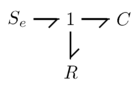
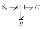
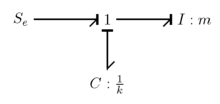
In bond graph notation, a causal stroke may be added to one end of the power bond to indicate that the opposite end is defining the effort. Consider a constant-torque motor driving a wheel, i.e. a source of effort (SE). That would be drawn as follows:

\begin{array}[b]{r}\text{motor}\\SE\end{array}\; \overset{\textstyle\tau}{\underset{\textstyle\omega}{-\!\!\!-\!\!\!-\!\!\!\rightharpoonup\!\!\!|}}\;\text{wheel}

Symmetrically, the side with the causal stroke (in this case the wheel) defines the flow for the bond.

Causality results in compatibility constraints. Clearly only one end of a power bond can define the effort and so only one end of a bond can have a causal stroke. In addition, the two passive components with time-dependent behavior, I and C, can only have one sort of causation: an I component determines flow; a C component defines effort. So from a junction, J, the preferred causal orientation is as follows:

J\; \overset{\textstyle}{\underset{\textstyle}{-\!\!\!-\!\!\!-\!\!\!\rightharpoonup\!\!\!|}}\;I \qquad\text{and}\qquad J\; \overset{\textstyle}{\underset{\textstyle}{|\!\!\!-\!\!\!-\!\!\!-\!\!\!\rightharpoonup}}\;C

The reason that this is the preferred method for these elements can be further analyzed if you consider the equations they would give shown by the tetrahedron of state.

$f(t)={\frac {1}{I}}\int e(t)\operatorname {d} \!t\qquad {\text{and}}\qquad e(t)={\frac {1}{C}}\int f(t)\operatorname {d} \!t$

The resulting equations involve the integral of the independent power variable. This is preferred over the result of having the causality the other way, which results in derivative. The equations can be seen below.

$e(t)=I\cdot {\dot {f}}(t)\qquad {\text{and}}\qquad f(t)=C\cdot {\dot {e}}(t)$

It is possible for a bond graph to have a casual bar on one of these elements in the non-preferred manner. In such a case a "casual conflict" is said to have occurred at that bond. The results of a causal conflict are only seen when writing the state-space equations for the graph. It is explained in more details in that section.

A resistor has no time-dependent behavior: apply a voltage and get a flow instantly, or apply a flow and get a voltage instantly, thus a resistor can be at either end of a causal bond:

J\; \overset{\textstyle}{\underset{\textstyle}{-\!\!\!-\!\!\!-\!\!\!\rightharpoonup\!\!\!|}}\;R \qquad \text{and} \qquad J\; \overset{\textstyle}{\underset{\textstyle}{|\!\!\!-\!\!\!-\!\!\!-\!\!\!\rightharpoonup}}\;R

Sources of flow (SF) define flow, sources of effort (SE) define effort. Transformers are passive, neither dissipating nor storing energy, so causality passes through them:

\;{\overset {\textstyle }{\underset {\textstyle }{-\!\!\!-\!\!\!-\!\!\!-\!\!\!-\!|}}}\;TF\;{\overset {\textstyle }{\underset {\textstyle }{-\!\!\!-\!\!\!-\!\!\!-\!\!\!-\!|}}}\;\qquad {\text{or}}\qquad \;{\overset {\textstyle }{\underset {\textstyle }{|\!\!\!-\!\!\!-\!\!\!-\!\!\!-\!\!\!-}}}\;TF\;{\overset {\textstyle }{\underset {\textstyle }{|\!\!\!-\!\!\!-\!\!\!-\!\!\!-\!\!\!-}}}\;

A gyrator transforms flow to effort and effort to flow, so if flow is caused on one side, effort is caused on the other side and vice versa:

$\;{\overset {\textstyle }{\underset {\textstyle }{|\!\!\!-\!\!\!-\!\!\!-\!\!\!-\!\!\!-}}}\;GY\;{\overset {\textstyle }{\underset {\textstyle }{-\!\!\!-\!\!\!-\!\!\!-\!\!\!-\!|}}}\;\qquad {\text{or}}\qquad \;{\overset {\textstyle }{\underset {\textstyle }{-\!\!\!-\!\!\!-\!\!\!-\!\!\!-\!|}}}\;GY\;{\overset {\textstyle }{\underset {\textstyle }{|\!\!\!-\!\!\!-\!\!\!-\!\!\!-\!\!\!-}}}\;$
Junctions

In a 0-junction, efforts are equal; in a 1-junction, flows are equal. Thus, with causal bonds, only one bond can cause the effort in a 0-junction and only one can cause the flow in a 1-junction. Thus, if the causality of one bond of a junction is known, the causality of the others is also known. That one bond is called the 'strong bond'

\text{strong bond}\rightarrow\;\dashv\!\overset{\textstyle \top}{\underset{\textstyle\bot}{0}}\!\dashv \qquad\text{and}\qquad \text{strong bond}\rightarrow\;\vdash\!\overset{\textstyle \bot}{\underset{\textstyle\top}{1}}\!\vdash

Determining causality

In order to determine the causality of a bond graph certain steps must be followed. Those steps are:

Draw Source Causal Bars
Draw Preferred causality for C and I bonds
Draw causal bars for 0 and 1 junctions, transformers and gyrators
Draw R bond causal bars
If a causal conflict occurs, change C or I bond to differentiation

A walk-through of the steps is shown below.

${\begin{matrix}S_{f}&{\overset {\textstyle }{\underset {\textstyle }{\!\!\!-\!\!\!-\!\!\!-\!\!\!\rightharpoonup }}}&0&{\overset {\textstyle }{\underset {\textstyle }{\!\!\!-\!\!\!-\!\!\!-\!\!\!\rightharpoonup }}}&TR&{\overset {\textstyle }{\underset {\textstyle }{\!\!\!-\!\!\!-\!\!\!-\!\!\!\rightharpoonup }}}&0&{\overset {\textstyle }{\underset {\textstyle }{\!\!\!-\!\!\!-\!\!\!-\!\!\!\rightharpoonup }}}&C_{5}\\&&\downharpoonleft &&^{r:1}&&\downharpoonleft &&\\&&C_{2}&&&&R_{6}&&\end{matrix}}$

The first step is to draw causality for the sources, over which there is only one. This results in the graph below.

${\begin{matrix}S_{f}&{\overset {\textstyle }{\underset {\textstyle }{|\!\!\!-\!\!\!-\!\!\!-\!\!\!\rightharpoonup }}}&0&{\overset {\textstyle }{\underset {\textstyle }{\!\!\!-\!\!\!-\!\!\!-\!\!\!\rightharpoonup }}}&TR&{\overset {\textstyle }{\underset {\textstyle }{\!\!\!-\!\!\!-\!\!\!-\!\!\!\rightharpoonup }}}&0&{\overset {\textstyle }{\underset {\textstyle }{\!\!\!-\!\!\!-\!\!\!-\!\!\!\rightharpoonup }}}&C_{5}\\&&\downharpoonleft &&^{r:1}&&\downharpoonleft &&\\&&C_{2}&&&&R_{6}&&\end{matrix}}$

The next step is to draw the preferred causality for the C bonds.

${\begin{matrix}S_{f}&{\overset {\textstyle }{\underset {\textstyle }{|\!\!\!-\!\!\!-\!\!\!-\!\!\!\rightharpoonup }}}&0&{\overset {\textstyle }{\underset {\textstyle }{\!\!\!-\!\!\!-\!\!\!-\!\!\!\rightharpoonup }}}&TR&{\overset {\textstyle }{\underset {\textstyle }{\!\!\!-\!\!\!-\!\!\!-\!\!\!\rightharpoonup }}}&0&{\overset {\textstyle }{\underset {\textstyle }{|\!\!\!-\!\!\!-\!\!\!-\!\!\!\rightharpoonup }}}&C_{5}\\&&{\bar {\downharpoonleft }}&&^{r:1}&&\downharpoonleft &&\\&&C_{2}&&&&R_{6}&&\end{matrix}}$

Next apply the causality for the 0 and 1 junctions, transformers, and gyrators.

${\begin{matrix}S_{f}&{\overset {\textstyle }{\underset {\textstyle }{|\!\!\!-\!\!\!-\!\!\!-\!\!\!\rightharpoonup }}}&0&{\overset {\textstyle }{\underset {\textstyle }{|\!\!\!-\!\!\!-\!\!\!-\!\!\!\rightharpoonup }}}&TR&{\overset {\textstyle }{\underset {\textstyle }{|\!\!\!-\!\!\!-\!\!\!-\!\!\!\rightharpoonup }}}&0&{\overset {\textstyle }{\underset {\textstyle }{|\!\!\!-\!\!\!-\!\!\!-\!\!\!\rightharpoonup }}}&C_{5}\\&&{\bar {\downharpoonleft }}&&^{r:1}&&{\underline {\downharpoonleft }}&&\\&&C_{2}&&&&R_{6}&&\end{matrix}}$

However, it should be noted that there is an issue with 0-junction on the left. The 0-junction has two causal bars at the junction, but the 0-junction wants one and only one at the junction. This was caused by having ${\textstyle C_{2}}$ be in the preferred causality. The only way to fix this is to flip that causal bar. This results in a causal conflict, the corrected version of the graph is below, with the ${\textstyle \star }$ representing the causal conflict.

${\begin{matrix}S_{f}&{\overset {\textstyle }{\underset {\textstyle }{|\!\!\!-\!\!\!-\!\!\!-\!\!\!\rightharpoonup }}}&0&{\overset {\textstyle }{\underset {\textstyle }{|\!\!\!-\!\!\!-\!\!\!-\!\!\!\rightharpoonup }}}&TR&{\overset {\textstyle }{\underset {\textstyle }{|\!\!\!-\!\!\!-\!\!\!-\!\!\!\rightharpoonup }}}&0&{\overset {\textstyle }{\underset {\textstyle }{|\!\!\!-\!\!\!-\!\!\!-\!\!\!\rightharpoonup }}}&C_{5}\\&&{\underline {\downharpoonleft }}\star &&^{r:1}&&{\underline {\downharpoonleft }}&&\\&&C_{2}&&&&R_{6}&&\end{matrix}}$

Converting from other systems

One of the main advantages of using bond graphs is that once you have a bond graph it doesn't matter the original energy domain. Below are some of the steps to apply when converting from the energy domain to a bond graph.

Electromagnetic

The steps for solving an Electromagnetic problem as a bond graph are as follows:

Place an 0-junction at each node
Insert Sources, R, I, C, TR, and GY bonds with 1 junctions
Ground (both sides if a transformer or gyrator is present)
Assign power flow direction
Simplify

These steps are shown more clearly in the examples below.

Linear mechanical

The steps for solving an Linear Mechanical problem as a bond graph are as follows:

Place 1-junctions for each distinct velocity (usually at a mass)
Insert R and C bonds at their own 0-junctions between the 1 junctions where they act
Insert Sources and I bonds on the 1 junctions where they act
Assign power flow direction
Simplify

These steps are shown more clearly in the examples below.

Simplifying

The simplifying step is the same regardless if the system was electromagnetic or linear mechanical. The steps are:

Remove Bond of zero power (due to ground or zero velocity)
Remove 0 and 1 junctions with less than three bonds
Simplify parallel power
Combine 0 junctions in series
Combine 1 junctions in series

These steps are shown more clearly in the examples below.

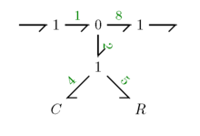
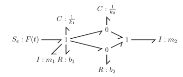
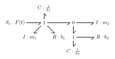
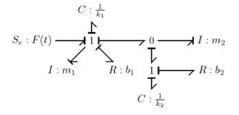
Parallel power

Parallel power is when power runs in parallel in a bond graph. An example of parallel power is shown below.

Parallel power can be simplified, by recalling the relationship between effort and flow for 0 and 1-junctions. To solve parallel power you will first want to write down all of the equations for the junctions. For the example provided, the equations can be seen below. (Please make note of the number bond the effort/flow variable represents).

${\begin{matrix}f_{1}=f_{2}=f_{3}&&e_{2}=e_{4}=e_{7}\\e_{1}=e_{2}+e_{3}&&f_{2}=f_{4}+f_{7}\\&&\\e_{3}=e_{5}=e_{6}&&f_{7}=f_{6}=f_{8}\\f_{3}=f_{5}+f_{6}&&e_{7}+e_{6}=e_{8}\end{matrix}}$

By manipulating these equations you can arrange them such that you can find an equivalent set of 0 and 1-junctions to describe the parallel power.

For example because ${\textstyle e_{3}=e_{6}}$ and ${\textstyle e_{2}=e_{7}}$ you can replace the variables in the equation ${\textstyle e_{1}=e_{2}+e_{3}}$ resulting in ${\textstyle e_{1}=e_{6}+e_{7}}$ and since

${\textstyle e_{6}+e_{7}=e_{8}}$ , we now know that $e_{1}=e_{8}$ . This relationship of two effort variables equaling can explained by an 0-junction. Manipulating other equations you can find that $f_{4}=f_{5}$ which describes the relationship of a 1-junction. Once you have determined the relationships that you need you can redraw the parallel power section with the new junctions. The result for the example show is seen below.

Examples

Simple electrical system

A simple electrical circuit consisting of a voltage source, resistor, and capacitor in series.

The first step is to draw 0-junctions at all of the node. The result is shown below.

${\begin{matrix}&0&&0&\\&&&&\\&&&&\\&0&&0&\end{matrix}}$

The next step is to add all of the elements acting at their own 1-junction. The result is below.

${\begin{matrix}&&&&R&&&&\\&&&&|&&&&\\&&0&-&1&-&0&&\\&&|&&&&|&&\\S_{e}&-&1&&&&1&-&C\\&&|&&&&|&&\\&&{\underline {0}}&-&-&-&0&&\end{matrix}}$

The next step is to pick a ground. The ground is simply an 0-junction that is going to be assumed to have no voltage. For this case, the ground will be chosen to be the lower left 0-junction, that is underlined above. The next step is to draw all of the arrows for the bond graph. The arrows on junctions should point towards ground (following a similar path to current). For resistance, inertance, and compliance elements, the arrows always point towards the elements. The result of drawing the arrows can be seen below, with the 0-junction marked with a star as the ground.

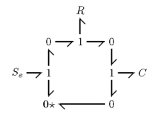
Now that we have the Bond graph, we can start the process of simplifying it. The first step is to remove all the ground nodes. Both of the bottom 0-junctions can be removed, because they are both grounded. The result is shown below.

Next, the junctions with less than three bonds can be removed. This is because flow and effort pass through these junctions without be modified, so they can be removed to allow us to draw less. The result can be seen below.

The final step is to apply causality to the bond graph. Applying causality was explained above. The final bond graph is shown below.

Advanced electrical system

A more advanced electrical system with a current source, resistors, capacitors, and a transformer

Following the steps with this circuit will result in the bond graph below, before it is simplified. The nodes marked with the star denote the ground.

Simplifying the bond graph will result in the image below.

Lastly, applying causality will result in the bond graph below. It should be noted that the bond with star denotes a causal conflict.

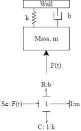
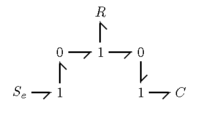
Simple linear mechanical

A simple linear mechanical system, consisting of a mass on a spring that is attached to a wall. The mass has some force being applied to it. An image of the system is shown below.

For a mechanical system, the first step is to place a 1-junction at each distant velocity, in this case there are two distant velocities, the mass and the wall. It is usually helpful to label the 1-junctions for reference. The result is below.

${\begin{matrix}&&\\&&\\1_{mass}&&\\&&\\&&\\&&\\1_{wall}&&\end{matrix}}$

The next step is to draw the R and C bonds at their own 0-junctions between the 1-junctions where they act. For this example there is only one of these bonds, the C bond for the spring. It acts between the 1-junction representing the mass and the 1-junction representing the wall. The result is below.

${\begin{matrix}&&\\&&\\1_{mass}&&\\|&&\\0&-&C:{\frac {1}{k}}\\|&&\\1_{wall}&&\end{matrix}}$

Next you want to add the sources and I bonds on the 1-junction where they act. There is one source, the source of effort (force) and one I bond, the mass of the mass both of which act on the 1-junction of the mass. The result is shown below.

${\begin{matrix}S_{e}:F(t)&&\\|&&\\1_{mass}&-&I:m\\|&&\\0&-&C:{\frac {1}{k}}\\|&&\\1_{wall}&&\end{matrix}}$

Next you want to assign power flow. Like the electrical examples, power should flow towards ground, in this case the 1-junction of the wall. Exceptions to this are R,C, or I bond, which always point towards the element. The resulting bond graph is below.

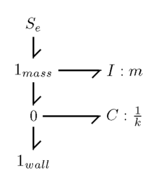
Now that the bond graph has been generated, it can be simplified. Because the wall is grounded (has zero velocity), you can remove that junction. As such the 0-junction the C bond is on, can also be removed because it will then have less than three bonds. The simplified bond graph can be seen below.

The last step is to apply causality, the final bond graph can be seen below.

Advanced linear mechanical

A more advanced linear mechanical system can be seen below.

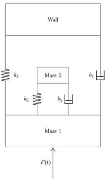
Just like the above example, the first step is to make 1-junctions at each of the distant velocities. In this example there are three distant velocity, Mass 1, Mass 2, and the wall. Then you connect all of the bonds and assign power flow. The bond can be seen below.

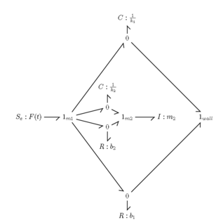
Next you start the process of simplifying the bond graph, by removing the 1-junction of the wall, and removing junctions with less than three bonds. The bond graph can be seen below.

It should be noted that there is parallel power in the bond graph. Solving parallel power was explained above. The result of solving it can be seen below.

Lastly, apply causality, the final bond graph can be seen below.

State equations

Once a bond graph is complete, it can be utilized to generate the state-space representation equations of the system. State-space representation is especially powerful as it allows complex multi-order differential system to be solved as a system of first-order equations instead. The general form of the state equation can be seen below.

${\dot {\textbf {x}}}(t)={\textbf {A}}\cdot {\textbf {x}}(t)+{\textbf {B}}\cdot {\textbf {u}}(t)$

Where, ${\textstyle {\textbf {x}}(t)}$ is a column matrix of the state variables, or the unknowns of the system. ${\textstyle {\dot {\textbf {x}}}(t)}$ is the time derivative of the state variables. ${\textstyle {\textbf {u}}(t)}$ is a column matrix of the inputs of the system. And ${\textstyle {\textbf {A}}}$ and ${\textstyle {\textbf {B}}}$ are matrices of constants based on the system. The state variables of a system are ${\textstyle q(t)}$ and ${\textstyle p(t)}$ values for each C and I bond without a causal conflict. Each I bond gets a ${\textstyle p(t)}$ while each C bond gets a ${\textstyle q(t)}$ .

For example, if you have the bond graph shown below.

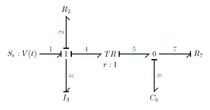
Would have the following ${\textstyle {\dot {\textbf {x}}}(t)}$ , ${\textstyle {\textbf {x}}(t)}$ , and ${\textstyle {\textbf {u}}(t)}$ matrices.

${\dot {\textbf {x}}}(t)=\left[{\begin{matrix}{\dot {p}}_{3}(t)\\{\dot {q}}_{6}(t)\end{matrix}}\right]\qquad {\text{and}}\qquad {\textbf {x}}(t)=\left[{\begin{matrix}p_{3}(t)\\q_{6}(t)\end{matrix}}\right]\qquad {\text{and}}\qquad {\textbf {u}}(t)=\left[{\begin{matrix}e_{1}(t)\end{matrix}}\right]$

The matrices of ${\textstyle {\textbf {A}}}$ and ${\textstyle {\textbf {B}}}$ are solved by determining the relationship of the state variables and their respective elements, as was described in the tetrahedron of state. The first step to solve the state equations, is to list all of the governing equations for the bond graph. The table below, shows the relationship between bonds and their governing equations.

	Bond Name	Bond with Causality	Governing Equation(s)
"♦" denotes preferred causality
One Port Elements	Source/ Sink, S	$S_{e}\;{\overset {\textstyle }{\underset {\textstyle }{-\!\!\!-\!\!\!-\!\!\!\rightharpoonup \!\!\!\|}}}\;$	$input=e(t)$
	Source/ Sink, S	$S_{f}\;{\overset {\textstyle }{\underset {\textstyle }{\|\!\!\!-\!\!\!-\!\!\!-\!\!\!\rightharpoonup }}}\;$	$input=f(t)$
	Resistance, R: Dissipated Energy	$\;{\overset {\textstyle }{\underset {\textstyle }{-\!\!\!-\!\!\!-\!\!\!\rightharpoonup \!\!\!\|}}}\ R$	$f(t)={\frac {1}{R}}\cdot e(t)$
	Resistance, R: Dissipated Energy	$\;{\overset {\textstyle }{\underset {\textstyle }{\|\!\!\!-\!\!\!-\!\!\!-\!\!\!\rightharpoonup }}}\ R$	$e(t)=R\cdot f(t)$
	Inertance, I: Kinetic Energy	♦ $\;{\overset {\textstyle }{\underset {\textstyle }{-\!\!\!-\!\!\!-\!\!\!\rightharpoonup \!\!\!\|}}}\ I$	$f(t)={\frac {1}{I}}\int e(t)\operatorname {d} \!t$
	Inertance, I: Kinetic Energy	$\;{\overset {\textstyle }{\underset {\textstyle }{\|\!\!\!-\!\!\!-\!\!\!-\!\!\!\rightharpoonup }}}\ I$	$e(t)=I\cdot {\dot {f}}(t)$
	Compliance, C: Potential Energy	$\;{\overset {\textstyle }{\underset {\textstyle }{-\!\!\!-\!\!\!-\!\!\!\rightharpoonup \!\!\!\|}}}\ C$	$f(t)=C\cdot {\dot {e}}(t)$
	Compliance, C: Potential Energy	♦ $\;{\overset {\textstyle }{\underset {\textstyle }{\|\!\!\!-\!\!\!-\!\!\!-\!\!\!\rightharpoonup }}}\ C$	$e(t)={\frac {1}{C}}\int f(t)\operatorname {d} \!t$
Two Port Elements	Transformer, TR	${\begin{matrix}{\overset {\textstyle }{{\underset {\textstyle }{\!\!\!-\!\!\!-\!\!\!-\!\!\!\rightharpoonup }}\|}}\ TR\ \ {\overset {\textstyle }{\underset {\textstyle }{\!\!\!-\!\!\!-\!\!\!-\!\!\!\rightharpoonup }}}\|\ \\^{r:1}\end{matrix}}$	$f_{1}r=f_{2}$ $e_{2}r=e_{1}$
	Transformer, TR	${\begin{matrix}\|\ {\overset {\textstyle }{\underset {\textstyle }{\!\!\!-\!\!\!-\!\!\!-\!\!\!\rightharpoonup }}}\ TR\ \ \|\ {\overset {\textstyle }{\underset {\textstyle }{\!\!\!-\!\!\!-\!\!\!-\!\!\!\rightharpoonup }}}\ \\^{r:1}\end{matrix}}$	$f_{1}r=f_{2}$ $e_{2}r=e_{1}$
	Gyrator, GY	${\begin{matrix}\|\ {\overset {\textstyle }{\underset {\textstyle }{\!\!\!-\!\!\!-\!\!\!-\!\!\!\rightharpoonup }}}\ GY{\overset {\textstyle }{\underset {\textstyle }{\!\!\!-\!\!\!-\!\!\!-\!\!\!\rightharpoonup }}}\|\ \\^{g:1}\end{matrix}}$	$f_{1}g=e_{2}$ $f_{2}g=e_{1}$
	Gyrator, GY	${\begin{matrix}\ {\overset {\textstyle }{\underset {\textstyle }{\!\!\!-\!\!\!-\!\!\!-\!\!\!\rightharpoonup }}}\|\ GY{\overset {\textstyle }{\underset {\textstyle }{\|\!\!\!-\!\!\!-\!\!\!-\!\!\!\rightharpoonup }}}\ \\^{g:1}\end{matrix}}$	$f_{1}g=e_{2}$ $f_{2}g=e_{1}$
Multi-port Elements	0 junction	One and only one causal bar at the junction	$all\ e(t)=$
	0 junction	One and only one causal bar at the junction	$\sum f(t)_{in}=\sum f(t)_{out}$
	1 junction	one and only one causal bar away from the junction	$\sum e(t)_{in}=\sum e(t)_{out}$
			$all\ f(t)=$

For the example provided,

The governing equations are the following.

${\begin{matrix}input=e_{1}&eq.1\\e_{1}=e_{2}+e_{3}+e_{4}&eq.2\\f_{1}=f_{2}=f_{3}=f_{4}&eq.3\\e_{2}=R_{2}\cdot f_{2}&eq.4\\f_{3}={\frac {1}{I_{3}}}\int e_{3}\operatorname {d} \!t={\frac {1}{I_{3}}}\cdot p_{3}&eq.5\\f_{4}\cdot r=f_{5}&eq.6\\e_{5}\cdot r=e_{4}&eq.7\\e_{5}=e_{6}=e_{7}&eq.8\\f_{5}=f_{6}+f_{7}&eq.9\\e_{6}={\frac {1}{C_{5}}}\int f_{6}\operatorname {d} \!t={\frac {1}{C_{6}}}\cdot q_{6}&eq.10\\f_{7}={\frac {1}{R_{7}}}\cdot e_{7}&eq.11\end{matrix}}$

These equations can be manipulated to yield the state equations. For this example, you are trying to find equations that relate ${\textstyle {\dot {p}}_{3}(t)}$ and ${\textstyle {\dot {q}}_{6}(t)}$ in terms of ${\textstyle p_{3}(t)}$ , ${\textstyle q_{6}(t)}$ , and ${\textstyle e_{1}(t)}$ .

To start you should recall from the tetrahedron of state that ${\textstyle {\dot {p}}_{3}(t)=e_{3}(t)}$ starting with equation 2, you can rearrange it so that $e_{3}=e_{1}-e_{2}-e_{4}$ . $e_{2}$ can be substituted for equation 4, while in equation 4, $f_{2}$ can be replaced by $f_{3}$ due to equation 3, which can then be replaced by equation 5. $e_4$ can likewise be replaced using equation 7, in which $e_{5}$ can be replaced with $e_{6}$ which can then be replaced with equation 10. Following these substituted yields the first state equation which is shown below.

${\dot {p}}_{3}(t)=e_{3}(t)=e_{1}(t)-{\frac {R_{2}}{I_{3}}}\cdot p_{3}(t)-{\frac {r}{C_{6}}}\cdot q_{6}(t)$

The second state equation can likewise be solved, by recalling that ${\textstyle {\dot {q}}_{6}(t)=f_{6}(t)}$ . The second state equation is shown below.

${\dot {q}}_{6}(t)=f_{6}(t)={\frac {r}{I_{3}}}\cdot p_{3}(t)-{\frac {1}{R_{7}\cdot C_{6}}}\cdot q_{6}(t)$

Both equations can further be rearranged into matrix form. The result of which is below.

${\begin{bmatrix}{\dot {p}}_{3}(t)\\{\dot {q}}_{6}(t)\end{bmatrix}}={\begin{bmatrix}-{\frac {R_{2}}{I_{3}}}&-{\frac {r}{C_{6}}}\\{\frac {r}{I_{3}}}&-{\frac {1}{R_{7}\cdot C_{6}}}\end{bmatrix}}{\begin{bmatrix}p_{3}(t)\\q_{6}(t)\end{bmatrix}}+{\begin{bmatrix}1\\0\end{bmatrix}}{\begin{bmatrix}e_{1}(t)\end{bmatrix}}$

At this point the equations can be treated as any other state-space representation problem.

International conferences on bond graph modeling (ECMS and ICBGM)

A bibliography on bond graph modeling may be extracted from the following conferences :

References

↑ Paynter, Henry M. (1961). Analysis and Design of Engineering Systems. The M.I.T. Press. ISBN 0-262-16004-8.
↑ "Bond Graph Modelling of Engineering Systems" (PDF).

Notes

↑ Bond graphs can also be used in thermal and chemical domains, but this is uncommon and won't be explained in this article.

Bond graph

Tetrahedron of state

Components

Single-port elements

Sources and sinks

Inertance

Resistance

Capacitance

Two-port elements

Transformer

Gyrator

Multi-port elements

0-junctions

1-junctions

Causality

Determining causality

Converting from other systems

Electromagnetic

Linear mechanical

Simplifying

Parallel power

Examples

Simple electrical system

Advanced electrical system

Simple linear mechanical

Advanced linear mechanical

State equations

International conferences on bond graph modeling (ECMS and ICBGM)

See also

References

Notes

Further reading