Bayes' theorem

A blue neon sign, showing the simple statement of Bayes’ theorem

In probability theory and statistics, Bayes’ theorem (alternatively Bayes’ law or Bayes' rule, also written as Bayes’s theorem) describes the probability of an event, based on prior knowledge of conditions that might be related to the event. For example, if cancer is related to age, then, using Bayes’ theorem, a person’s age can be used to more accurately assess the probability that they have cancer, compared to the assessment of the probability of cancer made without knowledge of the person's age.

One of the many applications of Bayes' theorem is Bayesian inference, a particular approach to statistical inference. When applied, the probabilities involved in Bayes' theorem may have different probability interpretations. With the Bayesian probability interpretation the theorem expresses how a subjective degree of belief should rationally change to account for availability of related evidence. Bayesian inference is fundamental to Bayesian statistics.

Bayes’ theorem is named after Reverend Thomas Bayes (/beɪz/; 1701–1761), who first provided an equation that allows new evidence to update beliefs in his An Essay towards solving a Problem in the Doctrine of Chances (1763). It was further developed by Pierre-Simon Laplace, who first published the modern formulation in his 1812 "Théorie analytique des probabilités". Sir Harold Jeffreys put Bayes’ algorithm and Laplace's formulation on an axiomatic basis. Jeffreys wrote that Bayes' theorem "is to the theory of probability what the Pythagorean theorem is to geometry".^[1]

Statement of theorem

Visualization of Bayes' theorem by superposition of two event tree diagrams.

Bayes' theorem is stated mathematically as the following equation:^[2]

P(A\mid B)={\frac {P(B\mid A)\,P(A)}{P(B)}},

where $A$ and $B$ are events and $P(B)\neq 0$ .

$P(A\mid B)$ is a conditional probability: the likelihood of event $A$ occurring given that $B$ is true.
$P(B\mid A)$ is also a conditional probability: the likelihood of event $B$ occurring given that $A$ is true.
$P(A)$ and $P(B)$ are the probabilities of observing $A$ and $B$ independently of each other; this is known as the marginal probability.

Examples

Drug testing

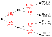
Tree diagram illustrating drug testing example. U, Ū, "+" and "−" are the events representing user, non-user, positive result and negative result. Percentages in parentheses are calculated.

Suppose that a test for using a particular drug is 99% sensitive and 99% specific. That is, the test will produce 99% true positive results for drug users and 99% true negative results for non-drug users. Suppose that 0.5% of people are users of the drug. What is the probability that a randomly selected individual with a positive test is a drug user?

{\begin{aligned}P({\text{User}}\mid {\text{+}})&={\frac {P({\text{+}}\mid {\text{User}})P({\text{User}})}{P(+)}}\\&={\frac {P({\text{+}}\mid {\text{User}})P({\text{User}})}{P({\text{+}}\mid {\text{User}})P({\text{User}})+P({\text{+}}\mid {\text{Non-user}})P({\text{Non-user}})}}\\[8pt]&={\frac {0.99\times 0.005}{0.99\times 0.005+0.01\times 0.995}}\\[8pt]&\approx 33.2\%\end{aligned}}

Even if an individual tests positive, it is more likely that they do not use the drug than that they do. This is because the number of non-users is large compared to the number of users. The number of false positives outweighs the number of true positives. For example, if 1000 individuals are tested, there are expected to be 995 non-users and 5 users. From the 995 non-users, 0.01 × 995 ≃ 10 false positives are expected. From the 5 users, 0.99 × 5 ≈ 5 true positives are expected. Out of 15 positive results, only 5 are genuine.

The importance of specificity in this example can be seen by calculating that even if sensitivity is raised to 100% and specificity remains at 99% then the probability of the person being a drug user only rises from 33.2% to 33.4%, but if the sensitivity is held at 99% and the specificity is increased to 99.5% then the probability of the person being a drug user rises to about 49.9%.

A more complicated example

The entire output of a factory is produced on three machines. The three machines account for 20%, 30%, and 50% of the factory output. The fraction of defective items produced is 5% for the first machine; 3% for the second machine; and 1% for the third machine. If an item is chosen at random from the total output and is found to be defective, what is the probability that it was produced by the third machine?

Once again, the answer can be reached without recourse to the formula by applying the conditions to any hypothetical number of cases. For example, if 100,000 items are produced by the factory, 20,000 will be produced by Machine A, 30,000 by Machine B, and 50,000 by Machine C. Machine A will produce 1000 defective items, Machine B 900, and Machine C 500. Of the total 2400 defective items, only 500, or 5/24 were produced by Machine C.

A solution is as follows. Let X_i denote the event that a randomly chosen item was made by the i ^th machine (for i = A,B,C). Let Y denote the event that a randomly chosen item is defective. Then, we are given the following information:

P(X_A) = 0.2, P(X_B) = 0.3, P(X_C) = 0.5.

If the item was made by the first machine, then the probability that it is defective is 0.05; that is, P(Y | X_A) = 0.05. Overall, we have

P(Y | X_A) = 0.05, P(Y | X_B) = 0.03, P(Y | X_C) = 0.01.

To answer the original question, we first find P(Y). That can be done in the following way:

P(Y) = Σ_i P(Y | X_i) P(X_i) = (0.05)(0.2) + (0.03)(0.3) + (0.01)(0.5) = 0.024.

Hence 2.4% of the total output of the factory is defective.

We are given that Y has occurred, and we want to calculate the conditional probability of X_C. By Bayes' theorem,

P(X_C | Y) = P(Y | X_C) P(X_C)/P(Y) = (0.01)(0.50)/0.024 = 5/24.

Given that the item is defective, the probability that it was made by the third machine is only 5/24. Although machine C produces half of the total output, it produces a much smaller fraction of the defective items. Hence the knowledge that the item selected was defective enables us to replace the prior probability P(X_C) = 1/2 by the smaller posterior probability P(X_C | Y) = 5/24.

Interpretations

A geometric visualisation of Bayes’ theorem. The figures denote the cells of the table involved in each metric, the probability being the fraction of each figure that is shaded. Similar reasoning shows that

{\begin{smallmatrix}P({\bar {A}}\mid B)\,=\,{\frac {P(B\mid {\bar {A}})\,P({\bar {A}})}{P(B)}}\end{smallmatrix}}

and so on.

The interpretation of Bayes’ theorem depends on the interpretation of probability ascribed to the terms. The two main interpretations are described below.

Bayesian interpretation

In the Bayesian (or epistemological) interpretation, probability measures a “degree of belief.” Bayes’ theorem then links the degree of belief in a proposition before and after accounting for evidence. For example, suppose it is believed with 50% certainty that a coin is twice as likely to land heads than tails. If the coin is flipped a number of times and the outcomes observed, that degree of belief may rise, fall or remain the same depending on the results.

For proposition A and evidence B,

P (A ), the prior, is the initial degree of belief in A.
P (A | B ), the posterior is the degree of belief having accounted for B.
the quotient P(B |A )/P(B) represents the support B provides for A.

For more on the application of Bayes’ theorem under the Bayesian interpretation of probability, see Bayesian inference.

Frequentist interpretation

Illustration of frequentist interpretation with tree diagrams. Bayes’ theorem connects conditional probabilities to their inverses.

In the frequentist interpretation, probability measures a “proportion of outcomes.” For example, suppose an experiment is performed many times. P(A) is the proportion of outcomes with property A, and P(B) that with property B. P(B | A ) is the proportion of outcomes with property B out of outcomes with property A, and P(A | B ) the proportion of those with A out of those with B.

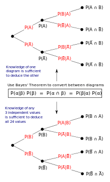
The role of Bayes’ theorem is best visualized with tree diagrams, as shown to the right. The two diagrams partition the same outcomes by A and B in opposite orders, to obtain the inverse probabilities. Bayes’ theorem serves as the link between these different partitionings.

Example

Tree diagram illustrating frequentist example. R, C, P and P bar are the events representing rare, common, pattern and no pattern. Percentages in parentheses are calculated. Note that three independent values are given, so it is possible to calculate the inverse tree (see figure above).

An entomologist spots what might be a rare subspecies of beetle, due to the pattern on its back. In the rare subspecies, 98% have the pattern, or P(Pattern | Rare) = 98%. In the common subspecies, 5% have the pattern. The rare subspecies accounts for only 0.1% of the population. How likely is the beetle having the pattern to be rare, or what is P(Rare | Pattern)?

From the extended form of Bayes’ theorem (since any beetle can be only rare or common),

{\begin{aligned}P({\text{Rare}}\mid {\text{Pattern}})&={\frac {P({\text{Pattern}}\mid {\text{Rare}})P({\text{Rare}})}{P({\text{Pattern}})}}\\[8pt]&={\frac {P({\text{Pattern}}\mid {\text{Rare}})P({\text{Rare}})}{P({\text{Pattern}}\mid {\text{Rare}})P({\text{Rare}})+P({\text{Pattern}}\mid {\text{Common}})P({\text{Common}})}}\\[8pt]&={\frac {0.98\times 0.001}{0.98\times 0.001+0.05\times 0.999}}\\[8pt]&\approx 1.9\%\end{aligned}}

Forms

Events

Simple form

For events A and B, provided that P(B) ≠ 0,

P(A\mid B)={\frac {P(B\mid A)\,P(A)}{P(B)}}\cdot

In many applications, for instance in Bayesian inference, the event B is fixed in the discussion, and we wish to consider the impact of its having been observed on our belief in various possible events A. In such a situation the denominator of the last expression, the probability of the given evidence B, is fixed; what we want to vary is A. Bayes’ theorem then shows that the posterior probabilities are proportional to the numerator:

P(A\mid B)\propto P(A)\cdot P(B\mid A)

(proportionality over A for given B).

The posterior is proportional to the prior times the likelihood.^[3]

If events A₁, A₂, ..., are mutually exclusive and exhaustive, i.e., one of them is certain to occur but no two can occur together, and we know their probabilities up to proportionality, then we can determine the proportionality constant by using the fact that their probabilities must add up to one. For instance, for a given event A, the event A itself and its complement ¬A are exclusive and exhaustive. Denoting the constant of proportionality by c we have

P(A\mid B)=c\cdot P(A)\cdot P(B\mid A){\text{ and }}P(\neg A\mid B)=c\cdot P(\neg A)\cdot P(B\mid \neg A).

Adding these two formulas we deduce that

1=c\cdot (P(B\mid A)\cdot P(A)+P(B\mid \neg A)\cdot P(\neg A)),

or

c={\frac {1}{P(B\mid A)\cdot P(A)+P(B\mid \neg A)\cdot P(\neg A)}}={\frac {1}{P(B)}}.

Alternative form

Another form of Bayes’ Theorem that is generally encountered when looking at two competing statements or hypotheses is:

P(A\mid B)={\frac {P(B\mid A)\,P(A)}{P(B\mid A)P(A)+P(B\mid \neg A)P(\neg A)}}.

For an epistemological interpretation:

For proposition A and evidence or background B,^[4]

$P(A)$ is the prior probability, is the initial degree of belief in A.
$P(\neg A)$ is the corresponding probability of the initial degree of belief against A, where $1-P(A)=P(\neg A)$
$P(B\mid A)$ is the conditional probability or likelihood, is the degree of belief in B, given that the proposition A is true.
$P(B\mid \neg A)$ is the conditional probability or likelihood, is the degree of belief in B, given that the proposition $\neg A$ is true.
$P(A\mid B)$ is the posterior probability, is the probability for A after taking into account B for and against A.

Extended form

Often, for some partition {A_j} of the sample space, the event space is given or conceptualized in terms of P(A_j) and P(B | A_j). It is then useful to compute P(B) using the law of total probability:

P(B)={\sum _{j}P(B\mid A_{j})P(A_{j})},

\Rightarrow P(A_{i}\mid B)={\frac {P(B\mid A_{i})\,P(A_{i})}{\sum \limits _{j}P(B\mid A_{j})\,P(A_{j})}}\cdot

In the special case where A is a binary variable:

P(A\mid B)={\frac {P(B\mid A)\,P(A)}{P(B\mid A)P(A)+P(B\mid \neg A)P(\neg A)}}\cdot

Random variables

Diagram illustrating the meaning of Bayes' theorem as applied to an event space generated by continuous random variables X and Y. Note that there exists an instance of Bayes' theorem for each point in the domain. In practice, these instances might be parametrized by writing the specified probability densities as a function of x and y.

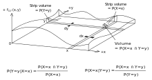
Consider a sample space Ω generated by two random variables X and Y. In principle, Bayes’ theorem applies to the events A = {X = x} and B = {Y = y}. However, terms become 0 at points where either variable has finite probability density. To remain useful, Bayes’ theorem may be formulated in terms of the relevant densities (see Derivation).

Simple form

If X is continuous and Y is discrete,

f_{X\,\mid \,Y=y}(x)={\frac {P(Y=y\mid X=x)\,f_{X}(x)}{P(Y=y)}}

where each $f$ is a density function.

If X is discrete and Y is continuous,

P(X=x\mid Y=y)={\frac {f_{Y\,\mid \,X=x}(y)\,P(X=x)}{f_{Y}(y)}}.

If both X and Y are continuous,

f_{X\,\mid \,Y=y}(x)={\frac {f_{Y\,\mid \,X=x}(y)\,f_{X}(x)}{f_{Y}(y)}}.

Extended form

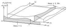
Diagram illustrating how an event space generated by continuous random variables X and Y is often conceptualized.

A continuous event space is often conceptualized in terms of the numerator terms. It is then useful to eliminate the denominator using the law of total probability. For f_Y(y), this becomes an integral:

f_{Y}(y)=\int _{-\infty }^{\infty }f_{Y}(y\mid X=\xi )\,f_{X}(\xi )\,d\xi .

Bayes’ rule

Bayes’ theorem in odds form is:

O(A_{1}:A_{2}\mid B)=O(A_{1}:A_{2})\cdot \Lambda (A_{1}:A_{2}\mid B)

where

\Lambda (A_{1}:A_{2}\mid B)={\frac {P(B\mid A_{1})}{P(B\mid A_{2})}}

is called the Bayes factor or likelihood ratio and the odds between two events is simply the ratio of the probabilities of the two events. Thus

O(A_{1}:A_{2})={\frac {P(A_{1})}{P(A_{2})}},

O(A_{1}:A_{2}\mid B)={\frac {P(A_{1}\mid B)}{P(A_{2}\mid B)}},

So the rule says that the posterior odds are the prior odds times the Bayes factor, or in other words, posterior is proportional to prior times likelihood.

Derivation

For events

Bayes’ theorem may be derived from the definition of conditional probability:

P(A\mid B)={\frac {P(A\cap B)}{P(B)}},{\text{ if }}P(B)\neq 0,

P(B\mid A)={\frac {P(B\cap A)}{P(A)}},{\text{ if }}P(A)\neq 0,

where $P(A\cap B)$ is the joint probability of both A and B being true, because

P(B\cap A)=P(A\cap B)

\Rightarrow P(A\cap B)=P(A\mid B)\,P(B)=P(B\mid A)\,P(A)

\Rightarrow P(A\mid B)={\frac {P(B\mid A)\,P(A)}{P(B)}},{\text{ if }}P(B)\neq 0.

For random variables

For two continuous random variables X and Y, Bayes’ theorem may be analogously derived from the definition of conditional density:

f_{X\,\mid \,Y=y}(x)={\frac {f_{X,Y}(x,y)}{f_{Y}(y)}}

f_{Y\,\mid \,X=x}(y)={\frac {f_{X,Y}(x,y)}{f_{X}(x)}}

Therefore

f_{X\,\mid \,Y=y}(x)={\frac {f_{Y\,\mid \,X=x}(y)\,f_{X}(x)}{f_{Y}(y)}}.

Correspondence to other mathematical frameworks

Propositional logic

Bayes' theorem represents a generalisation of contraposition which in propositional logic can be expressed as:

(\lnot A\to \lnot B)\to (B\to A).

The corresponding formula in terms of probability calculus is Bayes' theorem which in its expanded form is expressed as:

P(A\mid B)={\frac {P(B\mid A)\,a(A)}{P(B\mid A)\,a(A)+P(B\mid \lnot A)\,a(\lnot A)}}.

In the equation above the conditional probability $P(B\mid A)$ generalizes the logical statement $(A\to B)$ , i.e. in addition to assigning TRUE or FALSE we can also assign any probability to the statement. The term $a(A)$ denotes the prior probability (aka. the base rate) of $A$ . Assume that $P(A\mid B)=1$ is equivalent to $(B\to A)$ being TRUE, and that $P(A\mid B)=0$ is equivalent to $(B\to A)$ being FALSE. It is then easy to see that $P(A\mid B)=1$ when $P(\lnot B\mid \lnot A)=1$ i.e. when $(\lnot A\to \lnot B)$ is TRUE. This is because $P(B\mid \lnot A)=1-P(\lnot B\mid \lnot A)=0$ so that the fraction on the right-hand side of the equation above is equal to 1, and hence $P(A\mid B)=1$ which is equivalent to $(B\to A)$ being TRUE. Hence, Bayes' theorem represents a generalization of contraposition.^[5]

Subjective logic

Bayes' theorem represents a special case of conditional inversion in subjective logic expressed as:

(\omega _{A{\tilde {|}}B}^{S},\omega _{A{\tilde {|}}\lnot B}^{S})=(\omega _{B\mid A}^{S},\omega _{B\mid \lnot A}^{S})\,{\widetilde {\phi \,}}\,a_{A},\,

where $\,{\widetilde {\phi \,}}\,$ denotes the operator for conditional inversion. The argument $(\omega _{B\mid A}^{S},\omega _{B\mid \lnot A}^{S})$ denotes a pair of binomial conditional opinions, as expressed by source $S$ , and the argument $a_{A}$ denotes the prior probability (aka. the base rate) of $A$ . The pair of inverted conditional opinions is denoted $(\omega _{A{\tilde {|}}B}^{S},\omega _{A{\tilde {|}}\lnot B}^{S})$ . The conditional opinion $\omega _{A\mid B}^{S}$ generalizes the probabilistic conditional $P(A\mid B)$ , i.e. in addition to assigning a probability the source $S$ can assign any subjective opinion to the conditional statement $(A\mid B)$ . A binomial subjective opinion $\omega _{A}^{S}$ is the belief in the truth of statement $A$ with degrees of uncertainty, as expressed by source $S$ . Every subjective opinion has a corresponding projected probability $P(\omega _{A}^{S})$ . The projected probability of opinions applied to Bayes' theorem produces a homomorphism so that Bayes' theorem can be expressed in terms of the projected probabilities of opinions:

P(\omega _{A{\tilde {|}}B}^{S})={\frac {P(\omega _{B\mid A}^{S})\,a(A)}{P(\omega _{B\mid A}^{S})\,a(A)+P(\omega _{B\mid \lnot A}^{S})\,a(\lnot A)}}.

Hence, the subjective Bayes' theorem represents a generalization of Bayes' theorem.^[6]

History

Bayes’ theorem was named after Thomas Bayes (1701–1761), who studied how to compute a distribution for the probability parameter of a binomial distribution (in modern terminology). Bayes’ unpublished manuscript was significantly edited by Richard Price before it was posthumously read at the Royal Society. Price edited^[7] Bayes’ major work “An Essay towards solving a Problem in the Doctrine of Chances” (1763), which appeared in Philosophical Transactions,^[8] and contains Bayes’ Theorem. Price wrote an introduction to the paper which provides some of the philosophical basis of Bayesian statistics. In 1765, he was elected a Fellow of the Royal Society in recognition of his work on the legacy of Bayes.^[9]^[10]

The French mathematician Pierre-Simon Laplace reproduced and extended Bayes’ results in 1774, apparently unaware of Bayes’ work.^[11]^[12] The Bayesian interpretation of probability was developed mainly by Laplace.^[13]

Stephen Stigler suggested in 1983 that Bayes’ theorem was discovered by Nicholas Saunderson, a blind English mathematician, some time before Bayes;^[14]^[15] that interpretation, however, has been disputed.^[16] Martyn Hooper^[17] and Sharon McGrayne^[18] have argued that Richard Price's contribution was substantial:

By modern standards, we should refer to the Bayes–Price rule. Price discovered Bayes’ work, recognized its importance, corrected it, contributed to the article, and found a use for it. The modern convention of employing Bayes’ name alone is unfair but so entrenched that anything else makes little sense.^[18]

Notes

↑ Jeffreys, Harold (1973). Scientific Inference (3rd ed.). Cambridge University Press. p. 31. ISBN 978-0-521-18078-8.
↑ Stuart, A.; Ord, K. (1994), Kendall's Advanced Theory of Statistics: Volume I—Distribution Theory, Edward Arnold, §8.7
↑ Lee, Peter M. (2012). "Chapter 1". Bayesian Statistics. Wiley. ISBN 978-1-1183-3257-3.
↑ "Bayes' Theorem: Introduction". Trinity University.
↑ Audun Jøsang, 2016, Subjective Logic; A formalism for Reasoning Under Uncertainty. Springer, Cham, ISBN 978-3-319-42337-1
↑ Audun Jøsang, 2016, Generalising Bayes’ Theorem in Subjective Logic. IEEE International Conference on Multisensor Fusion and Integration for Intelligent Systems (MFI 2016), Baden-Baden, September 2016
↑ Richard Allen (1999). David Hartley on Human Nature. SUNY Press. pp. 243–4. ISBN 978-0-7914-9451-6. Retrieved 16 June 2013.
↑ Bayes, Thomas & Price, Richard (1763). "An Essay towards solving a Problem in the Doctrine of Chance. By the late Rev. Mr. Bayes, communicated by Mr. Price, in a letter to John Canton, A. M. F. R. S." (PDF). Philosophical Transactions of the Royal Society of London. 53 (0): 370–418. doi:10.1098/rstl.1763.0053.
↑ Holland, pp. 46–7.
↑ Richard Price (1991). Price: Political Writings. Cambridge University Press. p. xxiii. ISBN 978-0-521-40969-8. Retrieved 16 June 2013.
↑
Laplace refined Bayes’ theorem over a period of decades:
- Laplace announced his independent discovery of Bayes' theorem in: Laplace (1774) “Mémoire sur la probabilité des causes par les événements,” “Mémoires de l'Académie royale des Sciences de MI (Savants étrangers),” 4: 621–656. Reprinted in: Laplace, “Oeuvres complètes” (Paris, France: Gauthier-Villars et fils, 1841), vol. 8, pp. 27–65. Available on-line at: Gallica. Bayes’ theorem appears on p. 29.
- Laplace presented a refinement of Bayes’ theorem in: Laplace (read: 1783 / published: 1785) “Mémoire sur les approximations des formules qui sont fonctions de très grands nombres,” “Mémoires de l'Académie royale des Sciences de Paris,” 423–467. Reprinted in: Laplace, “Oeuvres complètes” (Paris, France: Gauthier-Villars et fils, 1844), vol. 10, pp. 295–338. Available on-line at: Gallica. Bayes’ theorem is stated on page 301.
- See also: Laplace, “Essai philosophique sur les probabilités” (Paris, France: Mme. Ve. Courcier [Madame veuve (i.e., widow) Courcier], 1814), page 10. English translation: Pierre Simon, Marquis de Laplace with F. W. Truscott and F. L. Emory, trans., “A Philosophical Essay on Probabilities” (New York, New York: John Wiley & Sons, 1902), page 15.
↑ Daston, Lorraine (1988). Classical Probability in the Enlightenment. Princeton Univ Press. p. 268. ISBN 0-691-08497-1.
↑ Stigler, Stephen M. (1986). The History of Statistics: The Measurement of Uncertainty before 1900. Harvard University Press, Chapter 3.
↑ Stigler, Stephen M (1983). "Who Discovered Bayes' Theorem?". The American Statistician. 37 (4): 290–296. doi:10.1080/00031305.1983.10483122.
↑ De Vaux, Richard; Velleman, Paul; Bock, David (2016). Stats, Data and Models (4 ed.). Pearson. pp. 380–381. ISBN 978-0-321-98649-8.
↑ Edwards, A. W. F. (1986). "Is the Reference in Hartley (1749) to Bayesian Inference?". The American Statistician. 40 (2): 109–110. doi:10.1080/00031305.1986.10475370.
↑ Hooper, Martyn (2013). "Richard Price, Bayes' theorem, and God". Significance. 10 (1): 36–39. doi:10.1111/j.1740-9713.2013.00638.x.
1 2 McGrayne, S. B. (2011). The Theory That Would Not Die: How Bayes’ Rule Cracked the Enigma Code, Hunted Down Russian Submarines & Emerged Triumphant from Two Centuries of Controversy. Yale University Press. ISBN 978-0-300-18822-6.

External links

Bayes’ theorem at Encyclopædia Britannica
The Theory That Would Not Die by Sharon Bertsch McGrayne New York Times Book Review by John Allen Paulos on 5 August 2011
Visual explanation of Bayes using trees (video)
Bayes’ frequentist interpretation explained visually (video)
Earliest Known Uses of Some of the Words of Mathematics (B). Contains origins of “Bayesian,” “Bayes’ Theorem,” “Bayes Estimate/Risk/Solution,” “Empirical Bayes,” and “Bayes Factor.”
Weisstein, Eric W. "Bayes' Theorem". MathWorld.
Bayes’ theorem at PlanetMath.org.
Bayes Theorem and the Folly of Prediction
A tutorial on probability and Bayes’ theorem devised for Oxford University psychology students
An Intuitive Explanation of Bayes' Theorem by Eliezer S. Yudkowsky

This article is issued from Wikipedia. The text is licensed under Creative Commons - Attribution - Sharealike. Additional terms may apply for the media files.

[1] Jeffreys, Harold (1973). Scientific Inference (3rd ed.). Cambridge University Press. p. 31. ISBN 978-0-521-18078-8.

[2] Stuart, A.; Ord, K. (1994), Kendall's Advanced Theory of Statistics: Volume I—Distribution Theory, Edward Arnold, §8.7

[3] Lee, Peter M. (2012). "Chapter 1". Bayesian Statistics. Wiley. ISBN 978-1-1183-3257-3.

[4] "Bayes' Theorem: Introduction". Trinity University.

[5] Audun Jøsang, 2016, Subjective Logic; A formalism for Reasoning Under Uncertainty. Springer, Cham, ISBN 978-3-319-42337-1

[6] Audun Jøsang, 2016, Generalising Bayes’ Theorem in Subjective Logic. IEEE International Conference on Multisensor Fusion and Integration for Intelligent Systems (MFI 2016), Baden-Baden, September 2016

[7] Richard Allen (1999). David Hartley on Human Nature. SUNY Press. pp. 243–4. ISBN 978-0-7914-9451-6. Retrieved 16 June 2013.

[Price1763-8] Bayes, Thomas & Price, Richard (1763). "An Essay towards solving a Problem in the Doctrine of Chance. By the late Rev. Mr. Bayes, communicated by Mr. Price, in a letter to John Canton, A. M. F. R. S." (PDF). Philosophical Transactions of the Royal Society of London. 53 (0): 370–418. doi:10.1098/rstl.1763.0053.

[Holland46-9] Holland, pp. 46–7.

[10] Richard Price (1991). Price: Political Writings. Cambridge University Press. p. xxiii. ISBN 978-0-521-40969-8. Retrieved 16 June 2013.

[11] Laplace refined Bayes’ theorem over a period of decades:
Laplace announced his independent discovery of Bayes' theorem in: Laplace (1774) “Mémoire sur la probabilité des causes par les événements,” “Mémoires de l'Académie royale des Sciences de MI (Savants étrangers),” 4: 621–656. Reprinted in: Laplace, “Oeuvres complètes” (Paris, France: Gauthier-Villars et fils, 1841), vol. 8, pp. 27–65. Available on-line at: Gallica. Bayes’ theorem appears on p. 29.

Laplace presented a refinement of Bayes’ theorem in: Laplace (read: 1783 / published: 1785) “Mémoire sur les approximations des formules qui sont fonctions de très grands nombres,” “Mémoires de l'Académie royale des Sciences de Paris,” 423–467. Reprinted in: Laplace, “Oeuvres complètes” (Paris, France: Gauthier-Villars et fils, 1844), vol. 10, pp. 295–338. Available on-line at: Gallica. Bayes’ theorem is stated on page 301.

See also: Laplace, “Essai philosophique sur les probabilités” (Paris, France: Mme. Ve. Courcier [Madame veuve (i.e., widow) Courcier], 1814), page 10. English translation: Pierre Simon, Marquis de Laplace with F. W. Truscott and F. L. Emory, trans., “A Philosophical Essay on Probabilities” (New York, New York: John Wiley & Sons, 1902), page 15.

[mwAqU] Laplace announced his independent discovery of Bayes' theorem in: Laplace (1774) “Mémoire sur la probabilité des causes par les événements,” “Mémoires de l'Académie royale des Sciences de MI (Savants étrangers),” 4: 621–656. Reprinted in: Laplace, “Oeuvres complètes” (Paris, France: Gauthier-Villars et fils, 1841), vol. 8, pp. 27–65. Available on-line at: Gallica. Bayes’ theorem appears on p. 29.

[mwAqg] Laplace presented a refinement of Bayes’ theorem in: Laplace (read: 1783 / published: 1785) “Mémoire sur les approximations des formules qui sont fonctions de très grands nombres,” “Mémoires de l'Académie royale des Sciences de Paris,” 423–467. Reprinted in: Laplace, “Oeuvres complètes” (Paris, France: Gauthier-Villars et fils, 1844), vol. 10, pp. 295–338. Available on-line at: Gallica. Bayes’ theorem is stated on page 301.

[mwAqo] See also: Laplace, “Essai philosophique sur les probabilités” (Paris, France: Mme. Ve. Courcier [Madame veuve (i.e., widow) Courcier], 1814), page 10. English translation: Pierre Simon, Marquis de Laplace with F. W. Truscott and F. L. Emory, trans., “A Philosophical Essay on Probabilities” (New York, New York: John Wiley & Sons, 1902), page 15.

[12] Daston, Lorraine (1988). Classical Probability in the Enlightenment. Princeton Univ Press. p. 268. ISBN 0-691-08497-1.

[13] Stigler, Stephen M. (1986). The History of Statistics: The Measurement of Uncertainty before 1900. Harvard University Press, Chapter 3.

[14] Stigler, Stephen M (1983). "Who Discovered Bayes' Theorem?". The American Statistician. 37 (4): 290–296. doi:10.1080/00031305.1983.10483122.

[Stats,_Data_and_Models-15] De Vaux, Richard; Velleman, Paul; Bock, David (2016). Stats, Data and Models (4 ed.). Pearson. pp. 380–381. ISBN 978-0-321-98649-8.

[16] Edwards, A. W. F. (1986). "Is the Reference in Hartley (1749) to Bayesian Inference?". The American Statistician. 40 (2): 109–110. doi:10.1080/00031305.1986.10475370.

[17] Hooper, Martyn (2013). "Richard Price, Bayes' theorem, and God". Significance. 10 (1): 36–39. doi:10.1111/j.1740-9713.2013.00638.x.

[mcgrayne2011theory-18] 1 2 McGrayne, S. B. (2011). The Theory That Would Not Die: How Bayes’ Rule Cracked the Enigma Code, Hunted Down Russian Submarines & Emerged Triumphant from Two Centuries of Controversy. Yale University Press. ISBN 978-0-300-18822-6.

Bayes' theorem

Statement of theorem

Examples

Drug testing

A more complicated example

Interpretations

Bayesian interpretation

Frequentist interpretation

Example

Forms

Events

Simple form

Alternative form

Extended form

Random variables

Simple form

Extended form

Bayes’ rule

Derivation

For events

For random variables

Correspondence to other mathematical frameworks

Propositional logic

Subjective logic

History

See also

Notes

Further reading

External links