ABC analysis
In materials management, the ABC analysis (or Selective Inventory Control) is an inventory categorization technique. ABC analysis divides an inventory into three categories—"A items" with very tight control and accurate records, "B items" with less tightly controlled and good records, and "C items" with the simplest controls possible and minimal records.
The ABC analysis provides a mechanism for identifying items that will have a significant impact on overall inventory cost,[1] while also providing a mechanism for identifying different categories of stock that will require different management and controls.
The ABC analysis suggests that inventories of an organization are not of equal value.[2] Thus, the inventory is grouped into three categories (A, B, and C) in order of their estimated importance.
'A' items are very important for an organization. Because of the high value of these 'A' items, frequent value analysis is required. In addition to that, an organization needs to choose an appropriate order pattern (e.g. 'just-in-time') to avoid excess capacity. 'B' items are important, but of course less important than 'A' items and more important than 'C' items. Therefore, 'B' items are intergroup items. 'C' items are marginally important.
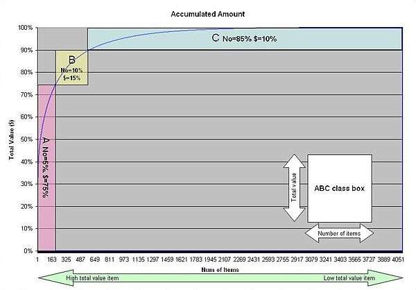
ABC analysis categories
There are no fixed threshold for each class, different proportion can be applied based on objective and criteria. ABC Analysis is similar to the Pareto principle in that the 'A' items will typically account for a large proportion of the overall value but a small percentage of the number of items.[3]
Examples of ABC class are
- 'A' items – 20% of the items accounts for 70% of the annual consumption value of the items
- 'B' items – 30% of the items accounts for 25% of the annual consumption value of the items
- 'C' items – 50% of the items accounts for 5% of the annual consumption value of the items
Another recommended breakdown of ABC classes:[4]
- "A" approximately 10% of items or 66.6% of value
- "B" approximately 20% of items or 23.3% of value
- "C" approximately 70% of items or 10.1% of value
ABC analysis in ERP packages
Major ERP packages have built-in function of ABC analysis. User can execute ABC analysis based on user defined criteria and system apply ABC code to items (parts).
Mathematical calculation of ABC analysis
Computed (calculated) ABC analysis delivers a precise mathematical calculation of the limits for the ABC classes.[5] It uses an optimization of cost (i.e. number of items) versus yield (i.e. sum of their estimated importance). Computed ABC was, for example, applied to feature selection for biomedical data,[6] business process management[7] and bankruptcy prediction.[8]
Example of the application of weighed operation based on ABC class
Actual distribution of ABC class in the electronics manufacturing company with 4051 active parts.
| ABC class | Number of items | Total amount required |
|---|---|---|
| A | 20% | 60% |
| B | 20% | 20% |
| C | 60% | 20% |
| Total | 100% | 100% |
Using this distribution of ABC class and change total number of the parts to 14213.
- Uniform purchase
When one applies equal purchasing policy to all 14213 components, example weekly delivery and re-order point (safety stock) of two weeks' supply assuming that there are no lot size constraints, the factory will have 16000 delivery in four weeks and average inventory will be 2½ weeks' supply.
| Uniform condition | Weighed condition | ||
|---|---|---|---|
| Items | Conditions | Items | Conditions |
| All items 14213 | Re-order point=2 weeks' supply Delivery frequency=weekly |
A-class items 200 | Re-order point=1 week's supply Delivery frequency=weekly |
| B-class items 400 | Re-order point=2 weeks' supply Delivery frequency=bi-weekly | ||
| C-class items 3400 | Re-order point=3 weeks' supply Delivery frequency=every 4 weeks | ||
- Weighed purchase
In comparison, when weighed purchasing policy applied based on ABC class, example C class monthly (every four weeks) delivery with re-order point of three weeks' supply, B class bi-weekly delivery with re-order point of 2 weeks' supply, A class weekly delivery with re-order point of 1 week's supply, total number of delivery in 4 weeks will be (A 200×4=800)+(B 400×2=800)+(C 3400×1=3400)=5000 and average inventory will be (A 75%×1.5weeks)+(B 15%x3 weeks)+(C 10%×3.5 weeks)=1.925 weeks' supply.
| ABC class | No of items | % of total value | Equal purchase | Weighed purchase | note | ||
|---|---|---|---|---|---|---|---|
| No of delivery in 4 weeks | average supply level | No of delivery in 4 weeks | average supply level | ||||
| A | 200 | 75% | 800 | 2.5 weeks | 800 | 1.5 weeksa | same delivery frequency, safety stock reduced from 2.5 to 1.5 weeksa, require tighter control with more man-hours. |
| B | 400 | 15% | 1600 | 2.5 weeks | 800 | 3 weeks | increased safety stock level by 20%, delivery frequency reduced to half. Fewer man-hours required. |
| C | 3400 | 10% | 13600 | 2.5 weeks | 3400 | 3.5 weeks | increased safety stock from 2.5 to 3.5 weeks' supply, delivery frequency is one quarter. Drastically reduced man-hour requirement. |
| Total | 4000 | 100% | 16000 | 2.5 weeks | 5000 | 1.925 weeks | average inventory value reduced by 23%, delivery frequency reduced by 69%. Overall reduction of man-hour requirement. |
a) A class item can be applied much tighter control like JIT daily delivery. If daily delivery with one day stock is applied, delivery frequency will be 4000 and average inventory level of A class item will be 1.5 days' supply and total inventory level will be 1.025 weeks' supply. reduction of inventory by 59%. Total delivery frequency also reduced to half from 16000 to 8200.
- Result
By applying weighed control based on ABC classification, required man-hours and inventory level are drastically reduced.
- Alternate way of finding ABC analysis:-
The ABC concept is based on Pareto's law.[9] If too much inventory is kept, the ABC analysis can be performed on a sample. After obtaining the random sample the following steps are carried out for the ABC analysis.
- Step 1: Compute the annual usage value for every item in the sample by multiplying the annual requirements by the cost per unit.
- Step 2: Arrange the items in descending order of the usage value calculated above.
- Step 3: Make a cumulative total of the number of items and the usage value.
- Step 4: Convert the cumulative total of the number of items and usage values into a percentage of their grand totals.
- Step 5: Draw a graph connecting cumulative % items and cumulative % usage value. The graph is divided approximately into three segments, where the curve sharply changes its shape. This indicates the three segments A, B and C.
See also
References
- ↑ Manufacturing planning and control systems for supply chain management By Thomas E. Vollmann
- ↑ Lun, Lai, Cheng (2010) Shipping and Logistics Management, p. 158
- ↑ Purchasing and Supply Chain Management By Kenneth Lysons, Brian Farrington
- ↑ Best Practice in Inventory Management, by Tony Wild (2nd Ed., p. 40)
- ↑ Ultsch, Alfred, Jörn Lötsch. "Computed ABC analysis for rational selection of most informative variables in multivariate data." PLOS One 10.6 (2015): e0129767.
- ↑ Kringel, D., Ultsch, A., Zimmermann, M., Jansen, J. P., Ilias, W., Freynhagen, R., ... & Resch, E. (2016). Emergent biomarker derived from next-generation sequencing to identify pain patients requiring uncommonly high opioid doses. The pharmacogenomics journal.
- ↑ Iovanella, A.: Vital few e trivial many, Il Punto, pp 10-13,July, 2017.
- ↑ Barbara Pawelek, Jozef Pociecha, Mateusz Baryla,ABC Anal-ysis in Corporate Bankruptcy Prediction, Abstracts of the IFCS Conference,p 17, Tokyo,Japan,2017
- ↑ Pareto's law in this example is that a few high usage value items constitute a major part of the capital invested in inventories whereas a large number of items having low usage value constitute an insignificant part of the capital.
External links
- SAP library ABC Analysis
- Oracle Overview of ABC Analysis
- ABC Analysis Solved Exercise