2D diagrams

• parameter is a variable on horizontal axis
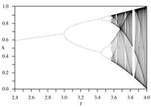
  • bifurcation diagram : P-curves ( = periodic points) versus parameter^[2]
  • orbit diagram : points of critical orbit versus parameter
  • skeleton diagram ( critical curves = q-curves)
  • Lyapunow diagram : Lyapunov exponent versus parameter^[3]
  • multiplier diagrams : multiplier of periodic orbit versus parameter
• constant parameter diagrams
  • cobweb diagram or a Verhulst diagram ^[4] = Graphical iteration
  • Iterates versus time diagram^[5] = connected scatter graph = time series
  • invariant density diagram , histogram,^[6] the distribution of the orbit,^[7] frequency distribution ^[8] = power spectrum ^[9]
  • Poincare plot^[10][11]

• 
  orbit diagram
• 
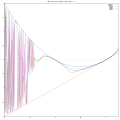  critical curves
• 
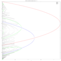  Bifurcation diagram for real quadratic map. Periodic points for periods 1,2,4,and 8 are shown
• 
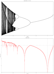  Orbit and Lyapunov diagrams
• 
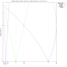  Multiplier diagram
• 
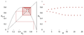  Logistic map cobweb and time evolution a=3.2

3D diagrams

• 
  An animated cobweb diagram
• 
  An animated connected scatter diagram

Tent map

Orbits of tent map:

• 
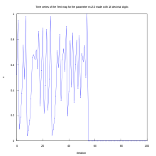  double precision computation and numerical error
• 
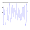  increased precision with no error

Logistic map

names :

• logistic map : ${\displaystyle f(x)=rx(1-x),}$
• logistic equation ${\displaystyle x_{n+1}=f(x_{n}),}$
• logistic difference equation ${\displaystyle x_{n+1}=rx_{n}(1-x_{n}),}$
• discrete dynamical system

The logistic map^[13][14] is defined by a recurrence relation ( difference equation) :

${\displaystyle x_{n+1}=rx_{n}(1-x_{n}),}$

where :

• ${\displaystyle r}$ is a given constant parameter
• ${\displaystyle x_{0}}$ is given the initial term
• ${\displaystyle x_{n}}$ is subsequent term determined by this relation

Do not confuse it with :

• differential equation ( which gives continous version )

Bash code ^[15] Javascript code from Khan Academy ^[16] MATLAB code:

r_values = (2:0.0002:4)';
iterations_per_value = 10;
y = zeros(length(r_values), iterations_per_value);
y0 = 0.5;
y(:,1) = r_values.*y0*(1-y0);
for i = 1:iterations_per_value-1
    y(:,i+1) = r_values.*y(:,i).*(1-y(:,i));
end
plot(r_values, y, '.', 'MarkerSize', 1);
grid on;

See also Lasin ^[17]

Maxima CAS code ^[18]

/* Logistic diagram by Mario Rodriguez Riotorto using Maxima CAS draw packag  */
pts:[];
for r:2.5 while r <= 4.0 step 0.001 do /* min r = 1 */
		(x: 0.25,
		for k:1 thru 1000 do x: r * x * (1-x), /* to remove points from image compute and do not draw it */
		for k:1 thru 500  do (x: r * x * (1-x), /* compute and draw it */
        	 	 pts: cons([r,x], pts))); /* save points to draw it later, re=r, im=x */
load(draw);
draw2d(	terminal   = 'png,
	file_name = "v",
        dimensions = [1900,1300],
	title      = "Bifurcation diagram, x[i+1] = r*x[i]*(1 - x[i])",
	point_type = filled_circle,
	point_size = 0.2,
	color = black,
	points(pts));

 ${\displaystyle x_{n}=sin^{2}(2^{n}arcsin{\sqrt {x_{0}}})}$

Better image

Bifurcation diagram of the logistic map

To show more detaile use tips by User:PAR:

"The horizontal axis is the r parameter, the vertical axis is the x variable. The image was created by forming a 1601 x 1001 array representing increments of 0.001 in r and x. A starting value of x=0.25 was used, and the map was iterated 1000 times in order to stabilize the values of x. 100,000 x -values were then calculated for each value of r and for each x value, the corresponding (x,r) pixel in the image was incremented by one. All values in a column (corresponding to a particular value of r) were then multiplied by the number of non-zero pixels in that column, in order to even out the intensities. Values above 250,000 were set to 250,000, and then the entire image was normalized to 0-255. Finally, pixels for values of r below 3.57 were darkened to increase visibility."

See also :

• tips from learner.org ^[21]

Real quadratic map

Lyapunov exponent - image and Maxima CAS code

Great images by Chip Ross^[25]

For ${\displaystyle x_{n+1}=x_{n}^{2}-c}$, the code in MATLAB can be written as:

c = (0:0.001:2)';
iterations_per_value = 100;
y = zeros(length(c), iterations_per_value);
y0 = 0;
y(:,1) = y0.^2 - c;
for i = 1:iterations_per_value-1
    y(:,i+1) = y(:,i).^2 - c;
end
plot(c, y, '.', 'MarkerSize', 1, 'MarkerEdgeColor', 'black');

Maxima CAS code for drawing real quadratic map : ${\displaystyle f_{c}(z)=z^{2}+c}$ :

/* based on the code by by Mario Rodriguez Riotorto */
pts:[];
for c:-2.0 while c <= 0.25 step 0.001 do 
                (x: 0.0,
                for k:1 thru 1000 do x: x * x+c, /* to remove points from image compute and do not draw it */
                for k:1 thru 500  do (x:  x * x+c, /* compute and draw it */
                         pts: cons([c,x], pts))); /* save points to draw it later, re=r, im=x */
load(draw);
draw2d( terminal   = 'svg,
        file_name = "b",
        dimensions = [1900,1300],
        title      = "Bifurcation diagram, x[i+1] = x[i]*x[i] +c",
        point_type = filled_circle,
        point_size = 0.2,
        color = black,
        points(pts));

program lapunow;

  { program draws bifurcation diagram y[n+1]=y[n]*y[n]+x,} { blue}
  {  x: -2 < x < 0.25 }
  {  y: -2 < y < 2    }
  {  and Lyapunov exponet for each x { white}

  uses crt,graph,
        { modul niestandardowy }
       bmpM, {screenCopy}
       Grafm;
  var xe,xemax,xe0,yemax,i1,i2:integer;
      yer,y,x,w,dx,lap:real;

  const xmin=-2;         { wspolczynnik   funkcji fx(y) }
        xmax=0.25;
        ymax=2;
        ymin=-2;
        i1max=100;            { liczba iteracji }
        i2max=20;
        lapmax=10;
        lapmin=-10;

   function wielomian2st(y,x:real) :real;
     begin
       wielomian2st:=y*y+x;
     end;  { wielomian2st }

  procedure wstep;
     begin
       opengraf;
       randomize;            { przygotowanie generatora liczb losowych }
       xemax:=getmaxx;              { liczba pixeli }
       yemax:=getmaxy;
       w:=(yemax+1)/(ymax-ymin);
       dx:=(xmax-xmin)/(xemax+1);
     end;

  begin {cialo}
    wstep;
    for xe:=xemax downTo 0 do
      begin {xe}
        x:=xmin+xe*dx;     { liniowe skalowanie x=a*xe+b }
        i1:=0;
        i2:=0;
        lap:=0;
        y:=random;        { losowy wybor    y0 : 0<y0<1 }

        while (abs(y)<ymax) and (i1<i1max)
        do
          begin {while i1}
            y:=wielomian2st(y,x);
            i1:=i1+1;
            lap:=lap+ln(abs(2*y)+0.1);
            if keypressed then halt;
          end; {while i1}

        while (i2<i2max) and (abs(y)<ymax)
         do
          begin   {while i2}
            y:=wielomian2st(y,x);
            yer:=(y-ymin)*w;         { skalowanie }
            putpixel(xe,yemax-round(yer),blue); { diagram bifurkacyjny }
            i2:=i2+1;
            lap:=lap+ln(abs(2*y)+0.1);
            if keypressed then halt;
          end; {while i2}

          lap:=lap/(i1max+i2max);
          yer:=(lap-lapmin)*(yemax+1)/(lapmax-lapmin);
          putpixel(xe,yemax-round(yer),white);         { wsp Lapunowa }
          putpixel(xe,yemax-round(-ymin*w),red);       { y=0 }
          putpixel(xe,yemax-round((1-ymin)*w),green);  { y=1}

      end; {xe}

    {..... os 0Y .......................................................}
    setcolor(red);
    xe0:=round((0-Xmin)/dx);     {xe0= xe : x=0 }
    line(xe0,0,xe0,yemax);
     SetColor(red);
    OutTextXY(XeMax-50,yemax-round((0-ymin)*w)+10,'y=0 ');
    SetColor(blue);
    OutTextXY(XeMax-50,yemax-round((1-ymin)*w)+10,'y=1');
    {....................................................................}
    screenCopy('screen',640,480);
    {}
    repeat until keypressed;
    closegraph;

 end.

{ Adam Majewski
Turbo Pascal 7.0  Borland
 MS-Dos / Microsoft}

self-similarity, scaling and renormalization

• Feigenbaums Scaling Law For TheLogistic Map ^[26]

See also

• Analytical properties of horizontal visibility graphs in the Feigenbaum scenario Bartolo Luque, Lucas Lacasa, Fernando J. Ballesteros, Alberto Robledo
• The Quadratic Map is Topologically Conjugate to the Shift Map - Gareth Roberts
• Numerical Errors in Logistic Map Calculation J. C. Sprott
• Numbers and Computers by Ronald T. Kneusel, Reviewed by David S. Mazel , on 01/27/2016
• Chaotic Modelling and Simulation Analysis of Chaotic Models, Attractors and Forms Christos H. Skiadas Charilaos Skiadas
• delayed_logistic
• The logistic map revisited Jerzy Ombach, Cracow, Poland
• Structure in the Parameter Dependence of Order and Chaos for the Quadratic Map Brian R. Hunt and Edward Ott
• Windows of periodicity scaling by Evgeny Demidov
• in Webgl by Ricky Reusser
• high-precision-feigenbaum-alpha-calc-using-julia by Stuart Brorson
• Feigenbaum Tree by 3DXM Consortium

software

• pynamical - Python package for modeling, simulating, visualizing, and animating discrete nonlinear dynamical systems and chaos

Videos:

• Illustration of Chaotic Systems Using Logistic Map by Zylasable
• Bifurcation Diagram for the Logistic Map Using R by Oxlajuj N'oj