Circuit

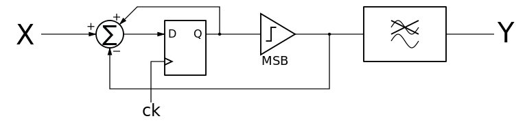
The first order ΣΔ modulator consists out of an accumulator and a comparator.

Modulator - first order - digital

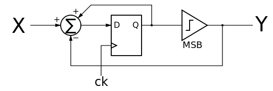
The output is a bit stream and the original signal can be reconstruted by the means of a lowpass filter.

Analysis

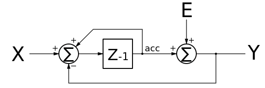
The frequency response of the sigma-delta modulator can be analysed by replacing the comparator with the addition of an error signal.

${\displaystyle {\begin{array}{ccl}z\cdot acc&=&X+acc-Y\\Y&=&acc+E\end{array}}}$

From these equations, one finds the Signal Transfer Funtion (STF)

${\displaystyle {\frac {Y(z)}{X(z)}}={\frac {1}{z}}}$

and the Noise Transfer Funtion (NTF)

${\displaystyle {\frac {Y(z)}{E(z)}}={\frac {z-1}{z}}}$

The STF is a one period delay but the NTF is a first order highpass function. This indicates that the modulation noise, due to the switching, occupies higher frequencies. If the input signal is limited to low frequencies, it is possible to separate the signal from the nois using a lowpass filter. As the highpass transfer function decreases by 20 dB/decade (or 6 dB/octave) as the frequency decreases, the signal to noise ratio increases by the same rate. Integrating the noise amplitude over the signal band shows that a first order modulator gains a signal to noise ration of 1.5 bit per octave. This can be compared to PCM which shows a gain of only 1 bit per octave.

When its input is constant, a first order modulator will provide a cyclic pattern. This pattern can become quite long for specific input values, and this leads to low-frequency ringing tones in the modulated signal. As these tones go lower in frequency, they become more and more difficult to separate from the original signal. Higher order modulators show less repetitive patterns and are thus preferred to first order ones.

Circuit

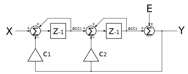
A second order ΣΔ modulator will require 2 accumulators. Different topologies are possible. The following circuit shows a typical second order circuit.

The 2 coefficients allow to control the digital to analog transfer function together with the corresponding noise shaping characteristic.

Analysis

Here too, the comparator can be replaced by the insertion of an error signal:

The NTF and STF can be found from the following equations:

${\displaystyle {\begin{array}{ccrcccccccccc}z\cdot {\begin{bmatrix}acc_{1}\\acc_{2}\end{bmatrix}}&=&{\begin{bmatrix}1&0\\1&1\end{bmatrix}}&\cdot &{\begin{bmatrix}acc_{1}\\acc_{2}\end{bmatrix}}&+&{\begin{bmatrix}1\\0\end{bmatrix}}&\cdot &X&+&{\begin{bmatrix}-c_{1}\\-c_{2}\end{bmatrix}}&\cdot &Y\\Y&=&{\begin{bmatrix}0&1\end{bmatrix}}&\cdot &{\begin{bmatrix}acc_{1}\\acc_{2}\end{bmatrix}}&+&{\begin{bmatrix}0\end{bmatrix}}&\cdot &X&+&{\begin{bmatrix}1\end{bmatrix}}&\cdot &E\end{array}}}$

which can be rewritten as:

${\displaystyle {\begin{array}{ccccccc}z\cdot {\overrightarrow {acc}}&=&\mathbf {A} \cdot {\overrightarrow {acc}}&+&\mathbf {B} \cdot X&+&\mathbf {B_{y}} \cdot y\\Y&=&\mathbf {C} \cdot {\overrightarrow {acc}}&+&\mathbf {D} \cdot X&+&\mathbf {D_{e}} \cdot E\end{array}}}$

Design

The poles of the STF are given by

${\displaystyle p_{12}=(1-{\frac {c_{2}}{2}})\pm j{\sqrt {c_{1}-{\frac {c_{2}^{2}}{4}}}}}$

This equation allows to arbitrarily place the poles of the STF. For a pair of poles at:

${\displaystyle p_{12}=a\pm jb}$

the modulator coefficients are:

${\displaystyle {\begin{cases}{\begin{array}{ll}c_{1}&=(1-a)^{2}+b^{2}\\c_{2}&=2(1-a)\end{array}}\end{cases}}}$

As an example, an all-pole Butterworth STF with cutoff frequency at 1/4 the sampling frequency give poles:

${\displaystyle p_{12}=0.375\pm j0.320}$

and coefficients:

${\displaystyle {\begin{cases}{\begin{array}{ll}c_{1}&=0.493\\c_{2}&=1.250\end{array}}\end{cases}}}$

An all-pole close to Bessel STF with cutoff frequency around 1/4 the sampling frequency give coefficients:

${\displaystyle {\begin{cases}{\begin{array}{ll}c_{1}&=26/32\\c_{2}&=56/32\end{array}}\end{cases}}}$

Note that the usual habits of using coefficients ${\displaystyle c_{1}=c_{2}=1}$ or ${\displaystyle c_{1}=c_{2}=1/2}$ both result in having poles exactly on the unit circle, which is not recommended in terms of stability.

Simplified Chain of Integrators with FeedBack (SCIFB)

The following picture shows a Simplified Chain of Integrators with FeedBack (SCIFB) modulator ^[2]:

Modulator SCIFB - order 3

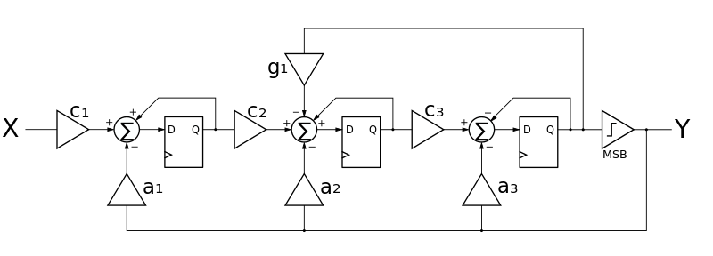
With coefficient ${\displaystyle g_{1}}$ different from zero, this is a structure with a local resonator.

For this structure, the system equations are:

${\displaystyle {\begin{array}{ccrcccccccccc}z\cdot {\begin{bmatrix}acc_{1}\\acc_{2}\\acc_{3}\end{bmatrix}}&=&{\begin{bmatrix}1&0&0\\c_{2}&1&-g_{1}\\0&c_{3}&1\end{bmatrix}}&\cdot &{\begin{bmatrix}acc_{1}\\acc_{2}\\acc_{3}\end{bmatrix}}&+&{\begin{bmatrix}c_{1}\\0\\0\end{bmatrix}}&\cdot &X&+&{\begin{bmatrix}-a_{1}\\-a_{2}\\-a_{3}\end{bmatrix}}&\cdot &Y\\Y&=&{\begin{bmatrix}0&0&1\end{bmatrix}}&\cdot &{\begin{bmatrix}acc_{1}\\acc_{2}\\acc_{3}\end{bmatrix}}&+&{\begin{bmatrix}0\end{bmatrix}}&\cdot &X&+&{\begin{bmatrix}1\end{bmatrix}}&\cdot &E\end{array}}}$

and the matrices are:

${\displaystyle {\begin{array}{ccc}A&=&{\begin{bmatrix}1&0&0\\c_{2}&1&-g_{1}\\0&c_{3}&1\end{bmatrix}}\end{array}}}$

${\displaystyle {\begin{array}{ccc}B&=&{\begin{bmatrix}c_{1}\\0\\0\end{bmatrix}}\end{array}}}$

${\displaystyle {\begin{array}{ccc}B_{y}&=&{\begin{bmatrix}-a_{1}\\-a_{2}\\-a_{3}\end{bmatrix}}\end{array}}}$

${\displaystyle {\begin{array}{ccc}C&=&{\begin{bmatrix}0&0&1\end{bmatrix}}\end{array}}}$

${\displaystyle {\begin{array}{ccc}D&=&{\begin{bmatrix}0\end{bmatrix}}\end{array}}}$

${\displaystyle {\begin{array}{ccc}D_{e}&=&{\begin{bmatrix}1\end{bmatrix}}\end{array}}}$

References

- ↑ Norsworthy, Steven R.; Schreier, Richard; Temes, Gabor C. (1997). Delta-Sigma Data Converters. IEEE Press. ISBN 0-7803-1045-4.
- ↑ Liu, Mingliang (2003), The Design of Delta-Sigma Modulators for Multi-Standard RF Receivers, http://scholarsarchive.library.oregonstate.edu/xmlui/handle/1957/30976