"[S]eparate the calculation phase from the colouring phase"—Claude Heiland-Allen
Theory

Introduction
- Your Friendly Guide to Colors in Data Visualisation by Lisa Charlotte Rost
- Playing with Gradient by rockraikar
- gimp concepts : gradients
- Ultra Fractal Gradient Hints by Janet Parke
- Image gradient at wikipedia
- Color gradient at wikipedia
- w3schools : css3 gradients
- gradients by Alan Gibson
- domain coloring
How to use color in your program
Steps:
- check your data ( type, range)
- choose what feature of the data you want to highlight
- apply gradient
- check the result/ optimize it
Transfer function
Transfer function T[1]

Examples: [2]
- gray(x) returns a shade of gray. The argument x should be in the range 0–1. If x=0, black is returned; if x=1, white is returned.
- rgb(r,g,b) returns a color with the specified RGB components, which should be in the range 0–1.
- cmyk(c,m,y,k) returns a color with the specified CMYK components, which should be in the range 0–1.
- hsb(h,s,b) returns a color with the specified coordinates in hue–saturation–brightness color space, which should be in the range 0–1.
- hsl(h,s,l)
Normalisation = resecale to standard range[3]
![{\displaystyle scalarvalue{\xrightarrow {normalize}}[0,1]{\xrightarrow {transferfunction}}colorvalue}](../../I/m/1add647e256d28424b7b58c806a2366fadcb4e77.svg)
Types:
- separated transfer functions for color and opacity in ParaView[4]
- Multi-Dimensional Transfer Functions[5]
- "The Transfer Function technique is a volume ray casting and rendering technique that assigns a different color and a different opacity/transparency value in different ranges of intensity values. This is done with a histogram based function, the "transfer function". The transfer function consists several control points, and each one of them corresponds to an intensity value and it has an RGB color and an opacity/transparency value. The intensity value of a control point is displayed with its color and opacity/transparency value, and the intensity values between two control points are displayed with the interpolated colors and the interpolated opacity/transparency values of the two control points. With the use of the transfer function, the different parts of the human body are displayed with a different color and a different opacity/transparency value." from Sante DICOM Viewer 3D Pro[6]
Color value
- color specification in Gnuplot
- colorhexa: Color encyclopedia : Information and conversion
- html color codes
- colour specifications by David Briggs
- Colour difference coding in computing (unfinished) by Billy Biggs
Color can be specified using one of the formats
- point in the space
- hex RGB
- hex RGBA
- rgb
- rgba
- hsl
- hsla
- cmyk
- name
Types of color gradient
Color gradients can be named by :
- dimension
- color model: hsv[7]
- number of segments of gradient
- function used to create gradient
- Number of colors
- gray scale precision in Gimp
- At integer precision
- An 8-bit integer grayscale image provides 255 available tonal steps from 0 (black) to 255 (white).
- A 16-bit integer grayscale image provides 65535 available tonal steps from 0 (black) to 65535 (white).
- A 32-bit integer grayscale image theoretically will provide 4294967295 tonal steps from 0 (black) to 4294967295 (white). But as high bit depth GIMP 2.10 does all internal processing at 32-bit floating point precision, the actual number of steps will be no more than the number of tonal steps available in a 32-bit floating point image.
- At floating point precision: the available number of tonal steps in a grayscale image depends on the specified bit depth (8-bit, 16-bit, or 32-bit)
- At integer precision
- gray scale precision in Gimp
Dimension
1D
Here color of pixel is proportional to 1D variable. For example in 2D space ( complex plane where point z = x+y*i) :
- position with respect to x-axis of Cartesian coordinate system : x
- distance to origin : r=abs(z)
- complex angle angle=arg(z)
An example of a function to return a color that is linearly between two given colors:
colorA = [0, 0, 255] # blue
colorB = [255, 0, 0] # red
function get_gradient_color(val):
# 'val' must be between 0 and 1
for i in [1,2,3]:
color[i] = colorA[i] + val * (colorB[i] - colorA[i])
return color
 1D gradient with color proportional to x
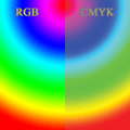 1D gradient with color proportional to radius
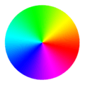 1D gradient with color proportional to angle
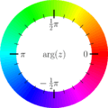 Hue circle for complex function plots
2D
ƒ(x) =(x2 − 1)(x − 2 − i)2/(x2 + 2 + 2i). The hue represents the function argument, while the saturation represents the magnitude.
Because color can be treated as more than 1D value it is used to represent more than one ( real or 1D) variable. For example :
- Robert Munafo uses 2 values from HSV model of color [8][9][10]
- John J. G. Savard uses own function [11][12]
- Domain coloring is a technique for visualizing functions of a complex variable
- matrixlab : rgb-images in MAtlab
- Multiwave coloring for Mandelbrot by Paul Derbyshire
' panomand/src/dll/fbmandel.bas
' https://www.unilim.fr/pages_perso/jean.debord/panoramic/mandel/panoramic_mandel.htm
' PANOMAND is an open source software for plotting Mandelbrot and Julia sets. It is written in two BASIC dialects: PANORAMIC and FreeBASIC
' by Jean Debord
' a simplified version of R Munafo's algorithm
' Color is defined in HSV space, according to Robert Munafo
' (http://mrob.com/pub/muency/color.html): the value V is
' computed from the distance estimator, while the hue H and
' saturation S are computed from the iteration number.

function MdbCol(byval Iter as integer, _
                byval mz   as double, _
                byref dz   as Complex) as integer
' Computes the color of a point
' Iter = iteration count
' mz   = modulus of z at iteration Iter
' dz   = derivative at iteration Iter

  if Iter = Max_Iter then return &HFFFFFF

  dim as double  lmz, mdz, Dist, Dwell, DScale, Angle, Radius, Q, H, S, V
  dim as integer R, G, B

  lmz = log(mz)
  mdz = CAbs(dz)

  ' Determine Value (luminosity) from Distance Estimator

  V = 1

  if mdz > 0 then
    Dist = pp * mz * lmz / mdz
    DScale = log(Dist / ScaleFact) / Lnp + Dist_Fact
    if DScale < -8 then
      V = 0
    elseif DScale < 0 then
      V = 1 + DScale / 8
    end if
  end if

  ' Determine Hue and Saturation from Continuous Dwell

  Dwell = Iter - log(lmz) / Lnp + LLE
  Q = log(abs(Dwell)) * AbsColor

  if Q < 0.5 then
    Q = 1 - 1.5 * Q
    Angle = 1 - Q
  else
    Q = 1.5 * Q - 0.5
    Angle = Q
  end if

  Radius = sqr(Q)

  if (Iter mod 2 = 1) and (Color_Fact > 0) then
    V = 0.85 * V
    Radius = 0.667 * Radius
  end if

  H = frac(Angle * 10)
  S = frac(Radius)

  HSVtoRGB H * 360, S, V, R, G, B
  return rgb(R, G, B)

end function
3D
- Hans Lundmark page[13]
Color model
Types :
- RGB is for the display
- CMYK is for printing
- other ( HSV, HSL, ...) are for choosing color
RGB
HSV
#include <stdio.h>
#include <stdlib.h>
#include <math.h>
#include <complex.h> // http://pubs.opengroup.org/onlinepubs/009604499/basedefs/complex.h.html

/*
based on
c++ program from :
http://commons.wikimedia.org/wiki/File:Color_complex_plot.jpg
by  	Claudio Rocchini

gcc d.c -lm -Wall

http://en.wikipedia.org/wiki/Domain_coloring

*/

const double PI = 3.1415926535897932384626433832795;
const double E  = 2.7182818284590452353602874713527;

/*

complex domain coloring
Given a complex number z=re^{ i \theta},

hue represents the argument ( phase, theta ),

sat and value represents the modulus

*/
int GiveHSV( double complex z, double HSVcolor[3] )
{
 //The HSV, or HSB, model describes colors in terms of hue, saturation, and value (brightness).

 // hue = f(argument(z))
 //hue values range from .. to ..
 double a = carg(z); //
 while(a<0) a += 2*PI; a /= 2*PI;

 // radius of z
 double m = cabs(z); //
 double ranges = 0;
 double rangee = 1;
 while(m>rangee){
   ranges = rangee;
   rangee *= E;
      }
 double k = (m-ranges)/(rangee-ranges);

 // saturation = g(abs(z))
 double sat = k<0.5 ? k*2: 1 - (k-0.5)*2;
 sat = 1 - pow( (1-sat), 3);
 sat = 0.4 + sat*0.6;

 // value = h(abs(z))
 double val = k<0.5 ? k*2: 1 - (k-0.5)*2;
   val = 1 - val;
   val = 1 - pow( (1-val), 3);
   val = 0.6 + val*0.4;

 HSVcolor[0]= a;
 HSVcolor[1]= sat;
 HSVcolor[2]= val;
return 0;
}


int GiveRGBfromHSV( double HSVcolor[3], unsigned char RGBcolor[3] ) {
        double r,g,b;
        double h; double s; double v;
        h=HSVcolor[0]; // hue
        s=HSVcolor[1]; //  saturation;
        v = HSVcolor[2]; // = value;

        if(s==0)
                r = g = b = v;
        else {
                if(h==1) h = 0;
                double z = floor(h*6);
                int i = (int)z;
                double f = (h*6 - z);
                double p = v*(1-s);
                double q = v*(1-s*f);
                double t = v*(1-s*(1-f));
                switch(i){
                        case 0: r=v; g=t; b=p; break;
                        case 1: r=q; g=v; b=p; break;
                        case 2: r=p; g=v; b=t; break;
                        case 3: r=p; g=q; b=v; break;
                        case 4: r=t; g=p; b=v; break;
                        case 5: r=v; g=p; b=q; break;
                }
        }
        int c;
        c = (int)(256*r); if(c>255) c = 255; RGBcolor[0] = c;
        c = (int)(256*g); if(c>255) c = 255; RGBcolor[1] = c;
        c = (int)(256*b); if(c>255) c = 255; RGBcolor[2] = c;
  return 0;
}

int GiveRGBColor( double complex z, unsigned char RGBcolor[3])
{
  static double HSVcolor[3];
  GiveHSV( z, HSVcolor );
  GiveRGBfromHSV(HSVcolor,RGBcolor);
  return 0;
}

//
double complex fun(double complex c ){
  return (cpow(c,2)-1)*cpow(c-2.0- I,2)/(cpow(c,2)+2+2*I);} //

int main(){
        // screen (integer ) coordinate
        const int dimx = 800; const int dimy = 800;
        // world ( double) coordinate
        const double reMin = -2; const double reMax =  2;
        const double imMin = -2; const double imMax =  2;
        //
        double stepX=(imMax-imMin)/(dimy-1);
        double stepY=(reMax-reMin)/(dimx-1);

        static unsigned char RGBcolor[3];
        FILE * fp;
        char *filename ="complex.ppm";
        fp = fopen(filename,"wb");
        fprintf(fp,"P6\n%d %d\n255\n",dimx,dimy);

        int i,j;
        for(j=0;j<dimy;++j){
                double im = imMax - j*stepX;
                for(i=0;i<dimx;++i){
                        double re = reMax - i*stepY;
                        double complex z= re + im*I; //
                        double complex v = fun(z); //
                        GiveRGBColor( v, RGBcolor);

                        fwrite(RGBcolor,1,3,fp);
                }
        }
        fclose(fp);
        printf("OK - file %s saved\n", filename);

        return 0;
}
In Basic :
' /panomand/src/dll/hsvtorgb.bas
' https://www.unilim.fr/pages_perso/jean.debord/panoramic/mandel/panoramic_mandel.htm
' PANOMAND is an open source software for plotting Mandelbrot and Julia sets. It is written in two BASIC dialects: PANORAMIC and FreeBASIC
' by Jean Debord
sub HSVtoRGB(byref H as double,  _
             byref S as double,  _
             byref V as double,  _
             byref R as integer, _
             byref G as integer, _
             byref B as integer)

' Convert RGB to HSV
' Adapted from http://www.cs.rit.edu/~ncs/color/t_convert.html
' R, G, B values are from 0 to 255
' H = [0..360], S = [0..1], V = [0..1]
' if S = 0, then H = -1 (undefined)

  if S = 0 then  ' achromatic (grey)
    R = V * 255
    G = R
    B = R
    exit sub
  end if

  dim as integer I
  dim as double  Z, F, P, Q, T
  dim as double  RR, GG, BB

  Z = H / 60     ' sector 0 to 5
  I = int(Z)
  F = frac(Z)
  P = V * (1 - S)
  Q = V * (1 - S * F)
  T = V * (1 - S * (1 - F))

  select case I
    case 0
      RR = V
      GG = T
      BB = P
    case 1
      RR = Q
      GG = V
      BB = P
    case 2
      RR = P
      GG = V
      BB = T
    case 3
      RR = P
      GG = Q
      BB = V
    case 4
      RR = T
      GG = P
      BB = V
    case 5
      RR = V
      GG = P
      BB = Q
  end select

  R = RR * 255
  G = GG * 255
  B = BB * 255
end sub
Function
One can use any function in each segment of gradient. Output of function is scaled to range of color component.
Number of colors
Number of color is determined by color depth : from 2 colors to 16 mln of colors.
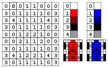
 6-bit RGB uniform palette with black borders
 Image:6-bit RGB uniform palette
 256 VGA color gradient
Repetition and offset
Direct repetition :
Color is proportional to position <0;1> of color in color gradient. if position > 1 then we have repetition of colors. it maybe useful
Mirror repetition :
"colorCycleMirror - This will reflect the colour gradient so that it cycles smoothly " [14]
Offset :
How to use color gradients in computer programs
First find what format of color you need in your program.[15][16]
Ways of making gradient :
- gradient functions
- gradient files
CLUT image
One can use CLUT image a a source of the gradient[21]
convert input.pgm -level 0,65532 clut.ppm -interpolate integer -clut -depth 8 output.png
CLUT Array
python
# http://jtauber.com/blog/2008/05/18/creating_gradients_programmatically_in_python/
# Creating Gradients Programmatically in Python by James Tauber

import sys

def write_png(filename, width, height, rgb_func):

    import zlib
    import struct
    import array

    def output_chunk(out, chunk_type, data):
        out.write(struct.pack("!I", len(data)))
        out.write(chunk_type)
        out.write(data)
        checksum = zlib.crc32(data, zlib.crc32(chunk_type))
        out.write(struct.pack("!I", checksum))

    def get_data(width, height, rgb_func):
        fw = float(width)
        fh = float(height)
        compressor = zlib.compressobj()
        data = array.array("B")
        for y in range(height):
            data.append(0)
            fy = float(y)
            for x in range(width):
                fx = float(x)
                data.extend([int(v * 255) for v in rgb_func(fx / fw, fy / fh)])
        compressed = compressor.compress(data.tostring())
        flushed = compressor.flush()
        return compressed + flushed

    out = open(filename, "w")
    out.write(struct.pack("8B", 137, 80, 78, 71, 13, 10, 26, 10))
    output_chunk(out, "IHDR", struct.pack("!2I5B", width, height, 8, 2, 0, 0, 0))
    output_chunk(out, "IDAT", get_data(width, height, rgb_func))
    output_chunk(out, "IEND", "")
    out.close()

def linear_gradient(start_value, stop_value, start_offset=0.0, stop_offset=1.0):
    return lambda offset: (start_value + ((offset - start_offset) / (stop_offset - start_offset) * (stop_value - start_value))) / 255.0

def gradient(DATA):
    def gradient_function(x, y):
        initial_offset = 0.0
        for offset, start, end in DATA:
            if y < offset:
                r = linear_gradient(start[0], end[0], initial_offset, offset)(y)
                g = linear_gradient(start[1], end[1], initial_offset, offset)(y)
                b = linear_gradient(start[2], end[2], initial_offset, offset)(y)
                return r, g, b
            initial_offset = offset
    return gradient_function

## EXAMPLES

# normally you would make these with width=1 but below I've made them 50
# so you can more easily see the result

# body background from jtauber.com and quisition.com
write_png("test1.png", 50, 143, gradient([
    (1.0, (0xA1, 0xA1, 0xA1), (0xDF, 0xDF, 0xDF)),
]))

# header background similar to that on jtauber.com
write_png("test2.png", 50, 90, gradient([
    (0.43, (0xBF, 0x94, 0xC0), (0x4C, 0x26, 0x4C)), # top
    (0.85, (0x4C, 0x26, 0x4C), (0x27, 0x13, 0x27)), # bottom
    (1.0,  (0x66, 0x66, 0x66), (0xFF, 0xFF, 0xFF)), # shadow
]))

# header background from pinax
write_png("test3.png", 50, 80, gradient([
    (0.72, (0x00, 0x26, 0x4D), (0x00, 0x40, 0x80)),
    (1.0,  (0x00, 0x40, 0x80), (0x00, 0x6C, 0xCF)), # glow
]))

# form input background from pinax
write_png("test4.png", 50, 25, gradient([
    (0.33, (0xDD, 0xDD, 0xDD), (0xF3, 0xF3, 0xF3)), # top-shadow
    (1.0,  (0xF3, 0xF3, 0xF3), (0xF3, 0xF3, 0xF3)),
]))
perl
# Perl code
# http://www.angelfire.com/d20/roll_d3_for_this/mandel-highorder/mandel-high.pl
# from perl High-order Mandelbrot program.
# Written by Christopher Thomas.
# Picture palette info.

my ($palsize);
my (@palette);

if(0)
{
# Light/dark colour banded palette.
# NOTE: This looks ugly, probably because the dark colours look muddy.
$palsize = 16;
@palette =
  ( "  255   0   0", "    0 112 112", "  255 128   0", "    0   0 128",
    "  224 224   0", "   64   0  96", "    0 255   0", "   96   0  64",
    "    0 224 224", "  128   0   0", "    0   0 255", "  128  64   0",
    "  128   0 192", "  112 112   0", "  192   0 128", "    0 128   0" );
}
else
{
# 8-colour rainbow palette.
$palsize = 8;
@palette =
  ( "  255   0   0", "  255 128   0",
    "  224 224   0", "    0 255   0",
    "    0 224 224", "    0   0 255",
    "  128   0 192", "  192   0 128" );
}
Conversions :
- between FractInt and Fractal eXtreme palettes [22]
lists:
Gradient functions
Name:
- coloring function
types
Examples :
- in JS using mandel.js[28] by Christopher Williams[29]
- Javascript using jQuery [30]
- C++ function by Richel Bilderbeek [31]
- Multiwave coloring for Mandelbrot[32]
- histogram colouring [33]
- Dave Green's `cubehelix' colour scheme
- css gradients
- stackoverflow question: how-to-create-colour-gradient-in-python
- complex_plot from Arb library and description
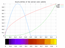
HSV gradient
Linear RGB gradient with 6 segments
- rainbow gradient
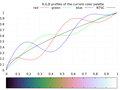
 2D RGB profile
 2D HSV profile
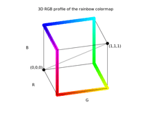 3D RGB profile
Rainbow gradient
- in scientific computing
Here gradient consists from 6 segments. In each segment only one RGB component of color is changed using linear function.
Delphi version
// Delphi version by Witold J.Janik with help Andrzeja Wąsika from [pl.comp.lang.delphi]
//  [i] changes from [iMin] to [iMax]

function GiveRainbowColor(iMin, iMax, i: Integer): TColor;
var
  m: Double;
  r, g, b, mt: Byte;
begin
  m := (i - iMin)/(iMax - iMin + 1) * 6;
  mt := (round(frac(m)*$FF));
  case Trunc(m) of
  0: begin
      R := $FF;
      G := mt;
      B := 0;
    end;
  1: begin
      R := $FF - mt;
      G := $FF;
      B := 0;
    end;
  2: begin
      R := 0;
      G := $FF;
      B := mt;
    end;
  3: begin
      R := 0;
      G := $FF - mt;
      B := $FF;
    end;
  4: begin
      R := mt;
      G := 0;
      B := $FF;
    end;
  5: begin
      R := $FF;
      G := 0;
      B := $FF - mt;
    end;
end; // case

  Result := rgb(R,G,B);
end;
/////
C version
Input of function are 2 variables :
- position of color in gradient, (a normalized float between 0.0 and 1.0 )
- color as an array of RGB components ( integer without sign from 0 to 255 )
This function does not use direct outoput ( void) but changes input variables color. One can use it this way:
GiveRainbowColor(0.25,color);
/* based on Delphi function by Witold J.Janik */
void GiveRainbowColor(double position,unsigned char c[])
{
  /* if position > 1 then we have repetition of colors it maybe useful    */

  if (position>1.0){if (position-(int)position==0.0)position=1.0; else position=position-(int)position;}


  unsigned char nmax=6; /* number of color segments */
  double m=nmax* position;

  int n=(int)m; // integer of m

  double f=m-n;  // fraction of m
  unsigned char t=(int)(f*255);


switch( n){
   case 0: {
      c[0] = 255;
      c[1] = t;
      c[2] = 0;
       break;
    };
   case 1: {
      c[0] = 255 - t;
      c[1] = 255;
      c[2] = 0;
       break;
    };
   case 2: {
      c[0] = 0;
      c[1] = 255;
      c[2] = t;
       break;
    };
   case 3: {
      c[0] = 0;
      c[1] = 255 - t;
      c[2] = 255;
       break;
    };
   case 4: {
      c[0] = t;
      c[1] = 0;
      c[2] = 255;
       break;
    };
   case 5: {
      c[0] = 255;
      c[1] = 0;
      c[2] = 255 - t;
       break;
    };
    default: {
      c[0] = 255;
      c[1] = 0;
      c[2] = 0;
       break;
    };

}; // case
}
Cpp version
// C++ version
// here are some my modification but the main code is the same
// as in Witold J.Janik code
//

Uint32 GiveRainbowColor(double position)

// this function gives 1D linear RGB color gradient
// color is proportional to position
// position  <0;1>
// position means position of color in color gradient

{
  if (position>1)position=position-int(position);
  // if position > 1 then we have repetition of colors
  // it maybe useful
  Uint8 R, G, B;// byte
  int nmax=6;// number of color bars
  double m=nmax* position;
  int n=int(m); // integer of m
  double f=m-n;  // fraction of m
  Uint8 t=int(f*255);


switch( n){
   case 0: {
      R = 255;
      G = t;
      B = 0;
       break;
    };
   case 1: {
      R = 255 - t;
      G = 255;
      B = 0;
       break;
    };
   case 2: {
      R = 0;
      G = 255;
      B = t;
       break;
    };
   case 3: {
      R = 0;
      G = 255 - t;
      B = 255;
       break;
    };
   case 4: {
      R = t;
      G = 0;
      B = 255;
       break;
    };
   case 5: {
      R = 255;
      G = 0;
      B = 255 - t;
       break;
    };

}; // case

  return (R << 16) | (G << 8) | B;
}
Sine based gradient
"The idea is to change the color based on a sine wave. This gives a nice smooth gradient effect (although it’s not linear, which is not a requirement anyway). By changing the frequency of the RGB components (we could theoretically work with other color spaces such as HSV) we can get various gradients. Also, we can also play with the phase of each color component, creating a “shifting” effect. The basic implementation of such a gradient can be implemented like so:"
/*
http://blogs.microsoft.co.il/pavely/2013/11/12/color-gradient-generator/


*/
public Color[] GenerateColors(int number) {
    var colors = new List<Color>(number);
    double step = MaxAngle / number;
    for(int i = 0; i < number; ++i) {
        var r = (Math.Sin(FreqRed * i * step + PhaseRed) + 1) * .5;
        var g = (Math.Sin(FreqGreen * i * step + PhaseGreen) + 1) * .5;
        var b = (Math.Sin(FreqBlue * i * step + PhaseBlue) + 1) * .5;
        colors.Add(Color.FromRgb((byte)(r * 255), (byte)(g * 255), (byte)(b * 255)));
    }
    return colors.ToArray();
}
"Where:
- the Freq* are the frequencies of the respective RGB colors
- Phase* are the phase shift values.
Note that all calculations are done with floating point numbers (ranging from 0.0 to 1.0), converting to a WPF Color structure (in this case) at the very end. This is simply convenient, as we’re working with trigonometric functions, which like floating point numbers rather than integers. The result is normalized to the range 0 to 1, as the sine function produces results from –1 to 1, so we add one to get a range of 0 to 2 and finally divide by 2 to get to the desired range."[37]
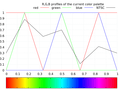
cubehelix
- Cubehelix gradient
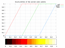
 2D RGB profile
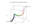 3D RGB profile
cubehelix gradient
/*
 GNUPLOT - stdfn.h
 Copyright 1986 - 1993, 1998, 2004   Thomas Williams, Colin Kelley
*/
#ifndef clip_to_01
#define clip_to_01(val)	\
    ((val) < 0 ? 0 : (val) > 1 ? 1 : (val))
#endif

/*
 input : position
 output : c array ( rgb color)

the colour scheme spirals (as a squashed helix) around the diagonal of the RGB colour cube

https://arxiv.org/abs/1108.5083
A colour scheme for the display of astronomical intensity images by D. A. Green
*/
void GiveCubehelixColor(double position, unsigned char c[]){


	/* GNUPLOT - color.h
	 * Petr Mikulik, December 1998 -- June 1999
	 * Copyright: open source as much as possible
	*/

	// t_sm_palette
  	/* gamma for gray scale and cubehelix palettes only */
  	double gamma = 1.5;

  	/* control parameters for the cubehelix palette scheme */
  	//set palette cubehelix start 0.5 cycles -1.5 saturation 1
	//set palette gamma 1.5
  	double cubehelix_start = 0.5;	/* offset (radians) from colorwheel 0 */
  	double cubehelix_cycles = -1.5;	/* number of times round the colorwheel */
  	double cubehelix_saturation = 1.0;	/* color saturation */
	double r,g,b;
	double gray = position;


	/*
 	 Petr Mikulik, December 1998 -- June 1999
 	* Copyright: open source as much as possible
 	*/
	// /* Map gray in [0,1] to color components according to colorMode */
	// function color_components_from_gray
	// from gnuplot/src/getcolor.c
	double phi, a;

	phi = 2. * M_PI * (cubehelix_start/3. +  gray * cubehelix_cycles);

	// gamma correction
	if (gamma != 1.0)    gray = pow(gray, 1./gamma);


	a = cubehelix_saturation * gray * (1.-gray) / 2.;

	// compute
	r = gray + a * (-0.14861 * cos(phi) + 1.78277 * sin(phi));
	g = gray + a * (-0.29227 * cos(phi) - 0.90649 * sin(phi));
	b = gray + a * ( 1.97294 * cos(phi));

	// normalize to [9,1] range
	r = clip_to_01(r);
	g = clip_to_01(g);
	b = clip_to_01(b);

	// change range to [0,255]
  	c[0] = (unsigned char) 255*r; //R
  	c[1] = (unsigned char) 255*g; // G
  	c[2] = (unsigned char) 255*b; // B

}
Gradient files
- Color Look-Up Table (CLUT)
File types for color gradient
There are special file types for color gradients:[38]
- The GIMP uses the files with .ggr extension [39]
- Fractint uses .map files [40]
- UltraFractal uses .ugr - These files can contain multiple gradients
- ual - old Ultra Fractal gradient file
- rgb, pal, gpf - gnuplot files
- The Matplotlib[41] colormap[42] is a lookup table[43]
- csv files
- maps in WHIP format ( Autodesk) by Paul Bourke
- Gnofract4D saves gradients only inside the graphic file, not as separate file.[44]
- MatLab
- Python
- R
- GMT
- QGIS
- Ncview
- Ferret
- Plotly
- Paraview
- VisIt
- Mathematica
- Surfer
- d3
- SKUA-GOCAD
- Petrel
- Fledermaus
- Qimera
- ImageJ
- Fiji
- Inkscape
csv files
a small table containing 33 values ( stored in a csv file) by Kenneth Moreland[45]
Scalar	R	G	B
0	59	76	192
0.03125	68	90	204
0.0625	77	104	215
0.09375	87	117	225
0.125	98	130	234
0.15625	108	142	241
0.1875	119	154	247
0.21875	130	165	251
0.25	141	176	254
0.28125	152	185	255
0.3125	163	194	255
0.34375	174	201	253
0.375	184	208	249
0.40625	194	213	244
0.4375	204	217	238
0.46875	213	219	230
0.5	221	221	221
0.53125	229	216	209
0.5625	236	211	197
0.59375	241	204	185
0.625	245	196	173
0.65625	247	187	160
0.6875	247	177	148
0.71875	247	166	135
0.75	244	154	123
0.78125	241	141	111
0.8125	236	127	99
0.84375	229	112	88
0.875	222	96	77
0.90625	213	80	66
0.9375	203	62	56
0.96875	192	40	47
1	180	4	38
CSS syntax
- css gradients
- linear
- non-repeating,
- repeating
- radial
- linear
Fractint map files
The default filetype extension for color-map files is ".MAP". These are ASCII text files. Consist of a series of RGB triplet values (one triplet per line, encoded as the red, green, and blue [RGB] components of the color). Color map ( or palette) is used as a colour look-up table[46] Default color map is in the Default.map file :
0 0 0            The default VGA color map
0 0 168
0 168 0
0 168 168
168 0 0
168 0 168
168 84 0
168 168 168
84 84 84
84 84 252
84 252 84
84 252 252
252 84 84
252 84 252
252 252 84
252 252 252
0 0 0
20 20 20
32 32 32
44 44 44
56 56 56
68 68 68
80 80 80
96 96 96
112 112 112
128 128 128
144 144 144
160 160 160
180 180 180
200 200 200
224 224 224
252 252 252
0 0 252
64 0 252
124 0 252
188 0 252
252 0 252
252 0 188
252 0 124
252 0 64
252 0 0
252 64 0
252 124 0
252 188 0
252 252 0
188 252 0
124 252 0
64 252 0
0 252 0
0 252 64
0 252 124
0 252 188
0 252 252
0 188 252
0 124 252
0 64 252
124 124 252
156 124 252
188 124 252
220 124 252
252 124 252
252 124 220
252 124 188
252 124 156
252 124 124
252 156 124
252 188 124
252 220 124
252 252 124
220 252 124
188 252 124
156 252 124
124 252 124
124 252 156
124 252 188
124 252 220
124 252 252
124 220 252
124 188 252
124 156 252
180 180 252
196 180 252
216 180 252
232 180 252
252 180 252
252 180 232
252 180 216
252 180 196
252 180 180
252 196 180
252 216 180
252 232 180
252 252 180
232 252 180
216 252 180
196 252 180
180 252 180
180 252 196
180 252 216
180 252 232
180 252 252
180 232 252
180 216 252
180 196 252
0 0 112
28 0 112
56 0 112
84 0 112
112 0 112
112 0 84
112 0 56
112 0 28
112 0 0
112 28 0
112 56 0
112 84 0
112 112 0
84 112 0
56 112 0
28 112 0
0 112 0
0 112 28
0 112 56
0 112 84
0 112 112
0 84 112
0 56 112
0 28 112
56 56 112
68 56 112
84 56 112
96 56 112
112 56 112
112 56 96
112 56 84
112 56 68
112 56 56
112 68 56
112 84 56
112 96 56
112 112 56
96 112 56
84 112 56
68 112 56
56 112 56
56 112 68
56 112 84
56 112 96
56 112 112
56 96 112
56 84 112
56 68 112
80 80 112
88 80 112
96 80 112
104 80 112
112 80 112
112 80 104
112 80 96
112 80 88
112 80 80
112 88 80
112 96 80
112 104 80
112 112 80
104 112 80
96 112 80
88 112 80
80 112 80
80 112 88
80 112 96
80 112 104
80 112 112
80 104 112
80 96 112
80 88 112
0 0 64
16 0 64
32 0 64
48 0 64
64 0 64
64 0 48
64 0 32
64 0 16
64 0 0
64 16 0
64 32 0
64 48 0
64 64 0
48 64 0
32 64 0
16 64 0
0 64 0
0 64 16
0 64 32
0 64 48
0 64 64
0 48 64
0 32 64
0 16 64
32 32 64
40 32 64
48 32 64
56 32 64
64 32 64
64 32 56
64 32 48
64 32 40
64 32 32
64 40 32
64 48 32
64 56 32
64 64 32
56 64 32
48 64 32
40 64 32
32 64 32
32 64 40
32 64 48
32 64 56
32 64 64
32 56 64
32 48 64
32 40 64
44 44 64
48 44 64
52 44 64
60 44 64
64 44 64
64 44 60
64 44 52
64 44 48
64 44 44
64 48 44
64 52 44
64 60 44
64 64 44
60 64 44
52 64 44
48 64 44
44 64 44
44 64 48
44 64 52
44 64 60
44 64 64
44 60 64
44 52 64
44 48 64
0 0 0
0 0 0
0 0 0
0 0 0
0 0 0
0 0 0
0 0 0
0 0 0
Gimp ggr files
"The gradients that are supplied with GIMP are stored in a system gradients folder. By default, gradients that you create are stored in a folder called gradients in your personal GIMP directory. Any gradient files (ending with the extension .ggr) found in one of these folders, will automatically be loaded when you start GIMP" ( from gimp doc ) Default gradients are in /usr/share/gimp/2.0/gradients directory ( check it in a window : Edit/preferences/directories)
Git repo
Gimp gradients can be created thru :
- GUI [47]
- manually in text editor ( use predefined gradients as a base)
- in own programs
Gimp gradient file format is described in:
- GIMP Application Reference Manual [48]
- source files :
- app/gradient.c and app/gradient_header.h for GIMP 1.3 version.[49]
- gimp-2.6.0/app/core/gimpgradient.c
Gimp Gradient Segment format :
typedef struct {
  gdouble                  left, middle, right;

  GimpGradientColor        left_color_type;
  GimpRGB                  left_color;
  GimpGradientColor        right_color_type;
  GimpRGB                  right_color;

  GimpGradientSegmentType  type;          /*  Segment's blending function  */
  GimpGradientSegmentColor color;         /*  Segment's coloring type      */

  GimpGradientSegment     *prev;
  GimpGradientSegment     *next;
} GimpGradientSegment;
In GimpConfig style format:[50]
<proposal>
# GIMP Gradient file

(GimpGradient "Abstract 1"
        (segment 0.000000 0.286311 0.572621
                (left-color (gimp-rgba 0.269543 0.259267 1.000000 1.000000))
                (right-color (gimp-rgba 0.215635 0.407414 0.984953 1.000000))
                (blending-function linear)
                (coloring-type rgb))
        (segment ...)
        ...
        (segment ...))
</proposal>
GIMP Gradient
Name: GMT_hot
3
0.000000 0.187500 0.375000 0.000000 0.000000 0.000000 1.000000 1.000000 0.000000 0.000000 1.000000 0 0
0.375000 0.562500 0.750000 1.000000 0.000000 0.000000 1.000000 1.000000 1.000000 0.000000 1.000000 0 0
0.750000 0.875000 1.000000 1.000000 1.000000 0.000000 1.000000 1.000000 1.000000 1.000000 1.000000 0 0
First line says it is a gimp gradient file.
Second line is a gradient's name.
Third line tells the number of segments in the gradient.
Each line following defines the property of each segment in following order :"[52]
- position of left stoppoint
- position of middle point
- position of right stoppoint
- R for left stoppoint
- G for left stoppoint
- B for left stoppoint
- A for left stoppoint
- R for right stoppoint
- G for right stoppoint
- B for right stoppoint
- A for right stoppoint
- Blending function constant
- coloring type constant
There are only two constants at the end of each line:
- the blending function constant of the segment (apparently 0=Linear, 1=Curved, 2=Sinusoidal, 3=Spherical (increasing), 4=Spherical (decreasing))
- the coloring type constant of the segment (probably 0=RGB, 1=HSV (counter-clockwise hue), 2=HSV (clockwise hue)[53]
json
links
- cpp code by Patrick Ross
- Reading gimp ggr files in python by Ned Batchelder
- Python Pil library functions for reading GIMP gradient files ( in file GimpGradientFile.py)
- perl scripts to convert gimp-1.2.x palettes and gradients into a 1.3 form by Jeff Trefftzs
- Gimp Python plugin: make-gradient.py by Giuseppe Conte
- gimp gradient files - lisp code from Polypen by Yannick Gingras
- Perl functions from GIMP pdb - gradient.pdb
- stackoverflow : javascript-color-gradient
- c pseudocode and js code by Christopher Williams
- Lode's Computer Graphics Tutorial : Light and Color
- bruce lindbloom : color equations
Collections of gradients / colormaps
- gradcentral
- Cpt-city
- gimp gradients (ggr files) are in directory : /usr/share/gimp/2.0/gradients/
- The COLOURlovers site hosts a million 5-colour palettes in several formats
- thi.ng
- SciVisColor
- Fabio Crameri: scientific colourmaps in provided in all major formats
programs
- gnuplot
- The CCC-Tool[54] is a general tool for the creation, analyzing and testing of colormaps with the effort to minimize the needed interaction components.
- image magic[55]
- OpenCV library
- matplotlib
- python
- math3d : sphere colormap
- gradient-converter-apophysis-to-kalles-fraktaler
tests
Test your :
- monitor ( gamut)
- graphic card
- printer
- own
Test your color abilities
- The X-Rite Color Challenge and Hue Test
- The FM100 Hue Test is an easy-to-administer test and a highly effective method for evaluating an individual's ability to discern color.
How to choose color gradient ?
- Nonlinear Color Scales for Interactive Exploration by Young Hyun
- gencolormap
- Color Maps for Scientific Visualization by Kenneth Moreland
- In Search of a Perfect Colormap by Peter Karpov
- Good Colour Maps: How to Design Them by Peter Kovesi
- Rainbow Color Map Critiques: An Overview and Annotated Bibliography By Steve Eddins, MathWorks
- scivis tutorials
- Matteo Niccoli
How to render light spectrum?
How to read(pick) color from the image ?
How to extract color palette from image ?
How to find lighter and darker colors based on any initial color ?
- 0to255 a color tool by Shaun Chapman uses the lightness (L) scale from HSL
- stackoverflow : formula-to-determine-brightness-of-rgb-color
- stackoverflow : programmatically-lighten-or-darken-a-hex-color-or-rgb-and-blend-colors
- learnwebgl: model_color by C. Wayne Brown: To change a color (r,g,b) to make it lighter, move it closer to (1,1,1). To change a color (r,g,b) to make it darker, move it closer to (0,0,0).
  // darker by C. Wayne Brown
  newR = R + (0-R)*t;  // where t varies between 0 and 1
  newG = G + (0-G)*t;  // where t varies between 0 and 1
  newB = B + (0-B)*t;  // where t varies between 0 and 1


  // lighter C. Wayne Brown
  newR = R + (1-R)*t;  // where t varies between 0 and 1
  newG = G + (1-G)*t;  // where t varies between 0 and 1
  newB = B + (1-B)*t;  // where t varies between 0 and 1
How to remove gradient banding ?
How to generate and refine palettes of optimally distinct colors
Gradient contours
- description by Alan Gibson.[60]
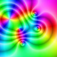
Examples of beatiful gradients
See also
- Image noise
- Commons Category:Color in computer graphics
- stackoverflow questions tagged gradient
- scratchapixel: simulating-sky
- Color by Bruce MacEvoy
- The X-Rite Color Challenge and Hue Test
- colour lovers: Color/s, Pattern/s, Palette/s, Lover/s or stats
- gamma correction
- coloring algorithms
References
- ↑ Basic Mapping Techniques from Computer Graphics Laboratory Department of Computer Science Zürich Switzerland
- ↑ pyxplot : color objects
- ↑ kitware : using-the-color-map-editor-in-paraview by Utkarsh Ayachit
- ↑ kitware : using-the-color-map-editor-in-paraview by Utkarsh Ayachit
- ↑ Visualization of Scalar Fields from IBBM
- ↑ santesoft : The Transfer Function technique
- ↑ dsp.stackexchange question: why-do-we-use-the-hsv-colour-space-so-often-in-vision-and-image-processing
- ↑ R2.1/2.C(1/2) by Robert Munafo
- ↑ Color by Robert Munafo
- ↑ Mandelbrot and Julia sets with PANORAMIC and FreeBASIC By jdebord
- ↑ The Mandelbrot Function by John J. G. Savard
- ↑ The Mandelbrot Function 2 by John J. G. Savard
- ↑ Visualizing complex analytic functions using domain coloring by Hans Lundmark
- ↑ The Fractal Explorer Pixel Bender filters by Tom Beddard
- ↑ What's Delphi TColor format? at ACASystems
- ↑ Delhi TColor at efg2.com
- ↑ wikipedia :Colour_look-up_table
- ↑ fractalforums : creating-a-good-palette-using-bezier-interpolation
- ↑ FracTest : palettes
- ↑ stefanbion : fraktal-generator and colormapping/
- ↑ Paul Tol's notes
- ↑ Fractal Forums > Fractal Software > Fractal Programs > Windows Fractal Software > Fractal eXtreme > Converting between FractInt and Fractal eXtreme palettes
- ↑ stackoverflow question : smooth-spectrum-for-mandelbrot-set-rendering
- ↑ on-rainbows by Charlie Loyd
- ↑ Stefan Bion : color mapping
- ↑ stackoverflow question : which-color-gradient-is-used-to-color-mandelbrot-in-wikipedia
- ↑ Making annoying rainbows in javascript A tutorial by jim bumgardner
- ↑ mandel.js by Christopher Williams
- ↑ Custom Palettes by Christopher Williams
- ↑ Gradient jQuery plugin Posted by David Wees
- ↑ C++ function by Richel Bilderbeek
- ↑ Multiwave coloring for Mandelbrot
- ↑ histogram colouring is really streching (not true histogram)
- ↑ Color by Robert Munafo
- ↑ Mandelbrot and Julia sets with PANORAMIC and FreeBASIC By Jean Debord
- ↑ c programs by Curtis T McMullen
- ↑ color-gradient-generator by Pavel
- ↑ Color gradient file formats explained
- ↑ GIMP add-ons: types, installation, management by Alexandre Prokoudine
- ↑ Fractint Palette Maps and map files
- ↑ matplotlib: colormap-manipulation
- ↑ matplotlib colormaps
- ↑ wikipedia: Lookup table
- ↑ gnofract4d manual
- ↑ kenneth moreland: color-maps
- ↑ w:Colour look-up table
- ↑ gimp-gradient-editor-dialog doc
- ↑ GimpGradient doc at GIMP Application Reference Manual
- ↑ [Gimp-developer] Format of GIMP gradient files
- ↑ [Gimp-developer] Format of GIMP gradient files
- ↑ [Gimp-developer] Format of GIMP gradient files
- ↑ gpr format description by Vinay S Raikar
- ↑ Emulating ggr/GIMP gradient in JavaFx
- ↑ CCC-Tool
- ↑ imagemagick : gradient
- ↑ extract color palletes from your favorite images by John Mangual
- ↑ algorithmia : create-a-custom-color-scheme-from-your-favorite-website/
- ↑ ImageMagick v6 Examples -- Color Quantization and Dithering
- ↑ Tool to extract palette / color table from image
- ↑ gradint contours by Alan Gibson