Introduction
The goal of the handbook is to outline the basic concepts about computer clusters. Firstly what exactly a cluster is and how to build a simple and clean cluster which provides a great starting point for more complex tasks. Also the handbook provides a guide for task scheduling and other important cluster management features. For the practical part most of the examples use Qlustar. Qlustar is a all-in-one cluster operating system that is easy to setup, extend and most importantly operate.
A computer cluster consists of a number of computers linked together, generally through local area networks (LANs). All the connected component-computers work closely together and in many ways as a single unit. One of the big advantages of computer clusters over single computers, are that they usually improves the performance greatly, while still being cheaper than single computers of comparable speed and size. Besides that a cluster provides in general larger storage capacity, better data integrity.
Nodes
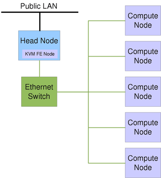
The term node usually describes one unit (linked computer) in a computer cluster. It represents the basic unit of a cluster. There a different types of notes like head-nodes, compute-, cloud- or storage-nodes. Nodes in a cluster are connected through dedicated internal Ethernet networks. The figure below shows a simple setup of the components building a basic HPC Cluster.
Software
The topic of this section is installation and maintenance of software that is not present in the default repositories of Ubuntu. Different methods to install, update and integrate software into the environment will be presented.
The Problem
Installing Software on GNU/Linux systems usually consists of three steps. The first step is downloading an archive which contains the source code of the application. After unpacking that archive, the code has to be compiled. Tools like Automake[1] assist the user in scanning the environment and making sure that all dependencies of the software are satisfied. In theory the software should be installed and ready to use after the three simple steps:
./configure./make./make install
Almost every provided README file in such an archive suggests doing this. Most of the time however, this procedure fails and the user has to manually solve issues. If all problems are solved, the code should be compiled (./make) and installed (./make install) (the second and third step). There are alternative projects to Automake like CMake[2] and WAF[3] that try to make the process less of a hassle. The process of installing and integrating software into an existing environment like this can take quite some time. If at some point the software has to receive an update, it is not guaranteed to take less time than the initial installation.
The root of this problem is that different distributions of GNU/Linux are generally quite diverse in the set of software that they provide after installation. This means if there are 5 different distributions, and you want to make sure that your software runs on each of them, you have to make sure that your software is compatible to potentially:
- 5 different versions of every library your software depends on.
- 5 different init systems (which take care of running daemons).
- 5 different conventions as to where software has to be installed.
Tools like Automake, CMake and WAF address this problem, but at the same time the huge diversity is also the reason why they are no 100% solutions and often fail.
Distribution Packages
Instead of trying to provide one archive that is supposed to run on every distribution of GNU/Linux it has become common to repackage software for each distribution. The repositories of Debian contain thousands of packages, that have been packaged solely for one release of Debian. This makes the installation and updating a breeze, but causes severe effort for the people who create these packages. Since Ubuntu is based on Debian most of these packages are also available for Ubuntu. These packages are pre-compiled, automatically install into the right location(s) and provide init scripts for the used init system. Installation of them is done by a package manager like apt or aptitude, which also manages future updates. There are only two minor problems:
- Software is packaged for a specific release of the distribution. For example Ubuntu 12.04 or Debian Squeeze. Once installed, usually only security updates are provided.
- Of course not every software is packaged and available in the default repositories.
This means, if you are using the latest long term support release of Ubuntu, most of the software you use is already over one year old and has since then, only received security updates. The reason for this is stability. Updates don’t always make everything better, sometimes they break stuff. If software A depends on software B it might not be compatible to a future release of B. But sometimes you really need a software update (for example to get support for newer hardware), or you just want to install software that is not available in the default repositories.
Personal Package Archives
For that reason Ubuntu provides a service called Personal Package Archives (PPA). It allows developers (or packagers) to create packages aimed at a specific release of Ubuntu for a specific architecture. These packages usually rely on the software available in the default repositories for that release, but could also rely on newer software available in other PPAs (uncommon). For users that means, they receive software that is easy to install, should not have dependency problems and is updated frequently with no additional effort. Obviously this is the preferred way to install software when compared to the traditional self compiling and installing.
How are PPAs used?
PPAs can be added by hand, but it is easier using the command add-apt-repository. That command is provided by the package python-software-properties.
- Listing 2.1: Install python-software-properties for the command add-apt-repository.
sudo apt-get install python-software-properties
The command add-apt-repository is used with the PPA name preceded by ppa:. An important thing to know is, that by installing such software you trust the packager that created the packages. It is advised to make sure that the packages won’t harm your system. The packager signsthe packages with his private key and also provides a public key. That public key is used by add-apt-repository to make sure that the packages have not been modified/manipulated since the packager created them. This adds security but as it was said before it does not protect you from malicious software that the packager might have included in the software.
- Listing 2.2: Add the ppa repository.
sudo add-apt-repository ppa:<ppa name>
After adding the repository you have to call apt-get update to update the package database. If you skip this step the software of the PPA won’t be available for installation.
- Listing 2.3: Update the package database.
sudo apt-get update
Now the software can be installed using apt-get insatll. It will also receive updated when apt-get upgrade is called. There is no extra step required to update software from PPAs.
- Listing 2.4: Install the desired packages.
sudo apt-get install <packages>
Qlustar
What is Qlustar?
Qlustar is a public HPC cluster operating system. It is based on Debian/Ubuntu. It is easy to you and highly customizable and do not need further packages to work. The installation of Qlustar has all necessary software to run a cluster.
Requirements
The requirements for the Qlustar OS are:
- A DVD or a USB flash-drive (minimum size 2GB) loaded with the Qlustar installer
- A 64bit x86 server/PC (or virtual machine) with
- at least two network adapters
- at least one disk with a minimum size of 160GB
- optionally a second (or more) disk(s) with a minimum size of 160GB
- CPU supporting virtualization (for virtual front-end and demo nodes)
- Working Internet connection
Installation process
Qlustar 9 provides an ISO install image that can be burned onto a DVD or be loaded onto an USB flash-drive. With that you can boot your machine from that DVD or drive. Choose “Qlustar installation” from the menu that will be presented when the server boots from you drive.

The kernel will be loaded and finally you can see a Qlustar welcome screen at which you can start the configuration process by pressen enter. In the first configuration screen select the desired localization settings. It’s important to set the right keyboard layout otherwise it will not function properly in the later setup process.

Select in the next screen the disk or disks to install Qlustar on. Make sure you have at least 160GB available space. The chosen disk will be used as a LVM physical volume to create a volume group.

For the home directories a separate file-system is used. When you have additional unused disks in the machine you can choose them. To have the home file-system on the same volume group choose the previously configured one. The option “Other” let’s you later setup a home file-system manually which is needed to add cluster users.

In the following screen you setup the network configuration. The number of compute nodes does not need to be exact and can be an approximate value. It determines the suggested cluster network address and other parameters. Also specify the mail relay and a root mail alias.
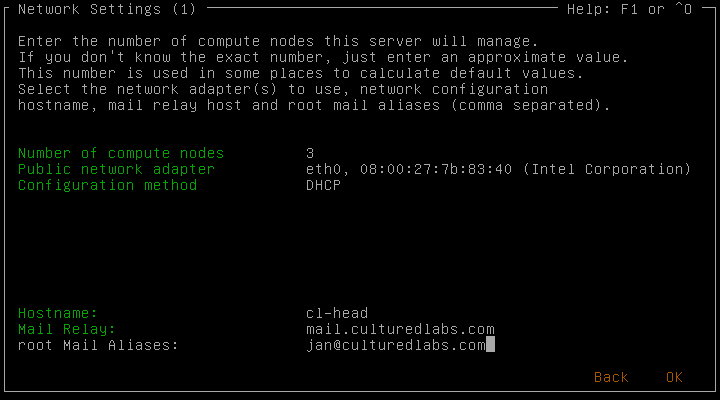
On the second network settings screen you can configure optional Infiniband and/or IPMI network parameters. The corresponding hardware wasn’t present in my particular cluster, so I chose accordingly.

To boost the stability and performance it is common practice to separate user from system activities as much as possible and so have a virtual front-end node for user access/activity. You can choose to setup this front-end node. To get all the necessary network pre-configurations it’s recommended to create a virtual demo-cluster. Lastly create a password for the root user.

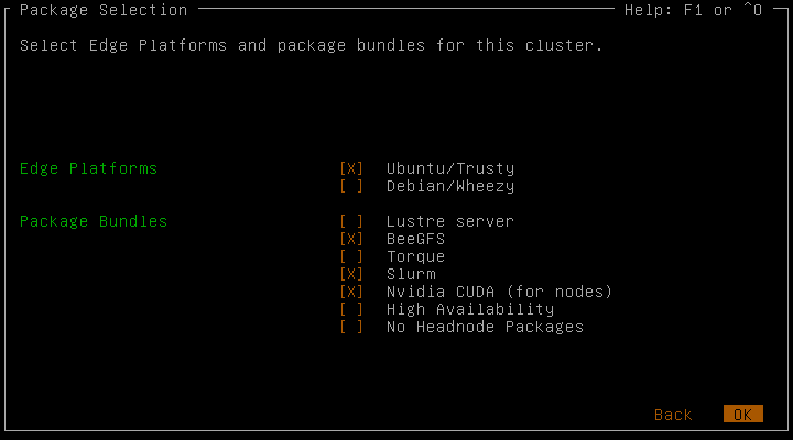
In the next screen you can select the preferred edge platforms. Multiple are possible and one is required. Choosing an edge platform will cause Qlustar images be based on it. Here you can also choose to install package bundles like Slurm (a popular workload manager/scheduler).
Before the actual installation process will start, you can review the installation settings. It shows a summary of the settings from the previous screens. Go back if there are any changes you want to make.

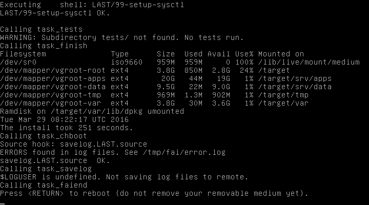
The completion of the installation can take up to a few minutes. Press enter at the end and reboot your machine after removing the installation DVD or USB.
First boot of the OS
Boot the newly installed Qlustar OS

and login as root with the password entered in the installation configuration. At the first start Qlustar isn’t configured completely yet. To start the post-install configuration process and complete the installation run the following command:
/usr/sbin/qlustar-initial-config

The last steps require you to name you cluster, setup NIS and configure ssh, QluMan and Slurm. Naming the cluster is easy, type any string you’d like. In the NIS setup and ssh configuration, just confirm the suggested settings to proceed. Qlustars management framework (QluMan) requires a mysql database. Here enter the password for the QluMan DB user. The whole initialization process can take some time. When the optional Slurm package was selected in the installation process, you need to generate a munge key and the specification of a password for the Slurm mysql account. When all the mentioned steps are completed make a final reboot.
With the command:
demo-system-start
you start the virtual demo-cluster (if chosen in to configure it at the installation). The configuration file “/etc/qlustar/vm-configs/demo-system.conf.” is used. Start a screen session by attaching to the console session of the virtual demo cluster nodes:
console-demo-vms

Now you have a base configuration of Qlustar with following services running: Nagios3, Ganglia, DHCP/ATFTP, NTP, (Slurm, if selected in the installation), NIS server, Mail service, MariaDB and QluMan. This is a powerful foundation for every cluster. If desired you can add more software at any time, create new users or get down to business by running QluMan, compiling MPI programs and run them.
Cluster Monitoring
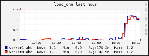
The topic of this chapter is cluster monitoring, a very versatile topic. There is plenty of software available to monitor distributed systems. However it is difficult to find one project that provides a solution for all needs. Among those needs may be the desire to efficiently gather as many metrics as possible about the utilization of “worker” nodes from a high performance cluster. Efficiency in this case is no meaningless advertising word – it is very important. Nobody wants to tolerate load imbalance just because some data to create graphs is collected, the priorities in high performance computing are pretty straight in that regard. Another necessity may be the possibility to observe certain things that are not allowed to surpass a specified threshold. Those things may be the temperature of water used for coolings things like CPUs or the allocated space on a hard disk drive. Ideally the monitoring software would have the possibility to commence counter-measures as long as the value is above the threshold. In the course this chapter two different monitoring solutions are be installed on a cluster of virtual machines. First, Icinga a fork of the widely used Nagios is be tested. After that Ganglia is used. Both solutions are Open Source and rather different in the functionalities they offer.

Figure 4.1 provides an overview of both the used cluster (of virtual machines) and the used software. All nodes use the most current Ubuntu LTS[4] release. In the case of Ganglia the software version is 3.5, the most current one and thus compiled from source. For Icinga version 1.8.4 is used.
Icinga
Icinga[5] is an Open Source monitoring solution. It is a fork of Nagios and maintains backwards compatibility. Thus all Nagios plugins also work with Icinga. The version provided by the official Ubuntu repositories in Ubuntu 12.04 is 1.6.1. To get a more current version the package provided by a Personal Package Archive (PPA) is used.[6]
Installation
Thanks to the provided PPA the installation was rather simple. There was only one minor nuisance. The official guide </ref> for installation using packages for Ubuntu suggested to install Icinga like this:
- Listing 4.1 Suggested order of packages to install Icinga on Ubuntu.
apt-get install icinga icinga-doc icinga-idoutils postgresql libdbd-pgsql postgresql-client
Unfortunately this failed, since the package installation of icinga-idoutils required a working database (either PostgreSQL or MySQL). So one has to switch the order of packages or just install PostgreSQL before Icinga.
Configuration
After the installation of Icinga the provided web interface was accessable right away (using port forwarding to access the virtual machine). Some plugins were enabled to monitor the host on which Icinga was installed by default.

Figure 4.2 shows the service status details for these plugins on the master node. Getting Icinga to monitor remote hosts (the worker nodes) required much more configuration. A look into the configuration folder of Icinga revealed how the master node was configured to display the information of figure [fig:default_plugins]. Information is split into two parts: host identification and service specification. The host identification consists of host_name, address and alias. A service is specified by a host_name, service_description and a check_command. The check_command accepts a Nagios plugin or a custom plugin which has to be configured in another Icinga configuration file: commands.cfg.

Figure 4.3 shows some important parts of the modified default configuration file used for the master node. As it can be seen both the host and service section start with a use statement which stands for the template that is going to be used. Icinga ships with a default (generic) template for hosts and services which is sufficient for us.

The question of how to achieve a setup as presented in figure 4.4 now arises. We want to use Icinga to monitor our worker nodes. For that purpose Icinga provides two different methods, which work the same way but use different techniques. In either case the Icinga running on the master node periodically asks the worker nodes for data. The other approach would have been, that Icinga just listens for data and the worker nodes initiate the communication themselves. The two different methods are SSH[7] and NRPE.[8] In the manuals both methods are compared and NRPE is recommended at the cost of increased configuration effort. NRPE causes less CPU overhead, SSH on the other hand is available on nearly every Linux machine and thus does not need to be configured. For our purpose decreased CPU overhead is a selling point and therefore NRPE is used. The next sections describe how Icinga has to be configured to monitor remote hosts with NRPE.
Master
In order to use NRPE additional software has to be installed on the master node. The package nagios-nrpe-plugin provides Icinga with the possibility to use NRPE to gather data from remote hosts. Unfortunately that package is part of Nagios and thus upon installation the whole Nagios project is supposed to be installed as a dependency. Luckily using the option –no-install-recommends for apt-get we can skip the installation of those packages. The now installed package provides a new check_command that can be used during the service definition for a new host: check_nrpe. That command can be used to execute a Nagios plugin or a custom command on a remote host. As figure [fig:flo_ahc_icinga_components] shows, we want to be able to check “gmond” (a deamon of the next monitoring solution: Ganglia) and if two NFS folders (/opt and /home) are mounted correctly. For that purpose we create a new configuration file /etc/icinga/objects, in this case worker1.cfg, and change the host section presented in figure [fig:host_service_config] to the hostname and IP of the desired worker. The check_command in the service section has to be used like this:
- Listing 4.2 NRPE check command in worker configuration file.
check_command check_nrpe_1arg!check-nfs-opt
The NRPE command accepts one argument (thus _1arg): a command that is going to be executed on the remote host specified in the host section. In this case that command is check-nfs-opt which not part of the Nagios plugin package, it is a custom shell script. The next section describes the necessary configuration on the remote host that has to be done before check-nfs-opt works.
Worker
Additional software has to be installed on the worker as well. In order to be able to respond to NRPE commands from the master the package nagios-nrpe-server has to be installed. That package provides Nagios plugins and a service that is answering the NRPE requests from the master. We are not going to use a Nagios plugin, instead we write three basic shell scripts that will make sure that (as shown in figure [fig:flo_ahc_icinga_components]):
- The
gmondservice of Ganglia is running. - Both
\optand\homeare correctly mounted using NFS from the master.
Before we can define those commands we have to allow the master to connect to our worker nodes:
- Listing 4.3 Add the IP address of the master to /
/etc/nagios/nrpe.cfg.
- Listing 4.3 Add the IP address of the master to /
allowed_hosts=127.0.0.1,!\colorbox{light-gray}{10.0.1.100}!
After that we can edit the file /etc/nagios/nrpe_local.cfg and add an alias and a path for the three scripts. The commands will be available to the master under the name of the specified alias.
- Listing 4.4 Add custom commands to
/etc/nagios/nrpe_local.cfg
- Listing 4.4 Add custom commands to
command[check-gmond-worker]=/opt/check-gmond.sh
command[check-nfs-home]=/opt/check-nfs-home.sh
command[check-nfs-opt]=/opt/check-nfs-opt.sh
This is all that has to be done on the worker. One can check if everything is setup correctly with a simple command from the master as listing [lst:nrpe_check] shows:
- Listing 4.5 Check if NRPE is setup correctly with
check_nrpe.
- Listing 4.5 Check if NRPE is setup correctly with
ehmke@master:/etc/icinga/objects$ /usr/lib/nagios/plugins/check_nrpe -H 10.0.1.2
CHECK_NRPE: Error - Could not complete SSL handshake.
Unfortunately in our case some extra steps were needed as the above command returned an error from every worker node. After turning on (and off again) the debug mode on the worker nodes (debug=1 in /etc/nagios/nrpe.cfg) the command returned the NRPE version and everything worked as expected. That is some strange behaviour, especially since it had to be done on every worker node.
- Listing 4.6
check_nrpesuccess!.
- Listing 4.6
ehmke@master:/etc/icinga/objects$ /usr/lib/nagios/plugins/check_nrpe -H 10.0.1.2
NRPE v2.12
Usage
Figure 4.5 shows the service status details for all hosts. Our custom commands are all working as expected. If that would not be the case they would appear as the ido2db process. The status of that service is critical which is visible at first glance. The Icinga plugin api[9] allows 4 different return statuses:
OKWARNINGCRITICALUNKNOWN
Additionally to the return code it is possible to return some text output. In our example we only return “Everything ok!”. The plugin which checks the ido2db process uses that text output to give a reason for the critical service status which is quite self-explanatory.

Ganglia
Ganglia is an open source distributed monitoring system specifically designed for high performance computing. It relies on RRDTool for data storage and visualization and available in all major distributions. The newest version added some interesting features which is why we did not use the older one provided by the official Ubuntu repositories.
Installation
The installation of Ganglia was pretty straightforward. We downloaded the latest packages for Ganglia[10] and RRDTool[11] which is used to generate the nice graphs. RRDTool itself also needed libconfuse to be installed. After the compilation (no special configure flags were set) and installation we had to integrate RRDTool into the environment such that Ganglia is able to use it. This usually means adjusting the environment variables PATH and LD_LIBRARY_PATH. Out of personal preference we choose another solution as listing [lst:rrd_env] shows.
- Listing 4.7 Integrating RRDTool into the environment..
echo '/opt/rrdtool-1.4.7/lib' >> /etc/ld.so.conf.d/rrdtool.conf
ldconfig
ln -s /opt/rrdtool-1.4.7/bin/rrdtool /usr/bin/rrdtool
Ganglia also needs libconfuse and additionally libapr. Both also have to be installed on the worker nodes. It was important to specify –with-gmetad during the configuration.
- Listing 4.8 Installation of Ganglia.
./configure --with-librrd=/opt/rrdtool-1.4.7 --with-gmetad --prefix=/opt/ganglia-3.5.0
make
sudo make install
Configuration

Ganglia consists of two major components: gmond and gmetad. Gmond is a monitoring daemon that has to run on every node that is supposed to be monitored. Gmetad is a daemon that polls other gmond daemons and stores their data in rrd databases which are then used to visualize the data in the Ganglia web interface. The goal was to configure Ganglia as shown in figure [fig:flo_ahc_ganglia_components]. The master runs two gmond daemons, one specifically for collecting data from the master, and the other one just to gather data from the gmond daemons running on the worker nodes. We installed Ganglia to /opt which is mounted on every worker via NFS. In order to start the gmond and gmetad processes on the master and worker nodes init scripts were used. The problem was, that there were no suitable init scripts provided by the downloaded tar ball. Our first idea was to extract the init script of the (older) packages of the Ubuntu repositories. That init script didn’t work as expected. Restarting and stopping the gmond service caused problems on the master node, since 2 gmond processes were running there. Instead of using the pid of the service they were killed by name, obviously no good idea. We tried to change the behaviour manually, but unfortunately that didn’t work. After the gmond process is started, the init systems reads the pid of the started service and stores it in a gmond.pid file. The problem was, that the gmond process demonizes after starting and changes the running user (from root to nobody). Those actions also changed the pid which means the .pid file is no longer valid and stopping and restarting the service won’t work. After a lot of trial and error we found a working upstart (the new init system used by Ubuntu) script in the most recent (not yet released) Ubuntu version 13.04. In that script we only had to adjust service names and make sure that the NFS partition is mounted before we start the service (start on (mounted MOUNTPOINT=/opt and runlevel [2345])). For some magical reason that setup even works on the master node with two gmond processes.
Master
At first we configured the gmetad daemon. We specified two data sources: “Infrastructure” (the master node) and “Cluster Nodes” (the workers). Gmetad gathers the data for these sources from the two running gmond processes on the master. To prevent conflicts both are accepting connections on different ports: 8649 (Infrastructure) and 8650 (Cluster Nodes). We also adjusted the grid name and the directory in which the rrd databases are stored.
- Listing 4.9 Interesting parts of
gmetad.conf.
- Listing 4.9 Interesting parts of
data_source "Infrastructure" localhost:8649
data_source "Cluster Nodes" localhost:8650
gridname "AHC Cluster"
rrd_rootdir "/opt/ganglia/rrds"
The next step was to configure the gmond processes on the master: gmond_master and gmond_collector. Since the gmond_master process doesn’t communicate with other gmond’s no communication configuration was necessary. We only had to specify a tcp_accept_channel on which the gmond responds to queries of gmetad. Additionally one can specify names for the host, cluster and owners and provide a location (for example the particular rack).
- Listing 4.10 Configuration of
gmond_master.conf.
- Listing 4.10 Configuration of
tcp_accept_channel {
    port = 8649
}
The gmond_collector process needs to communicate with the four gmond_worker processes. There are two different communications methods present in ganglia: unicast and multicast. We choose unicast and the setup was easy. The gmond_collector process additionally has to accept queries from the gmetad process which is why we specified another tcp_accept_channel. On the specified udp_recv_channel the gmond_collector waits for data from the gmond_worker processes.
- Listing 4.11 Configuration of
gmond_collector.conf.
- Listing 4.11 Configuration of
tcp_accept_channel {
    port = 8650
}
udp_recv_channel {
    port = 8666
}
Worker
The gmond_worker processes neither listens to other gmond processes nor accepts queries from a gmetad daemon. Thus the only interesting part in the configuration file is the sending mechanism of that gmond daemon.
Listing 4.12 Configuration of gmond_worker.conf.
udp_send_channel {
    host = master
    port = 8666
    ttl = 1
}
Usage
Ganglia already gathers and visualizes data about the cpu, memory, network and storage by default. It is also possible to extend the monitoring capabilities with custom plugins. The gathered data can be viewed in many small graphs each only featuring one data source, or in larger aggregated “reports”.

The front page of ganglia shows many of those aggregated reports for the whole grid and the “sub clusters”. Figure 4.7 shows that front page from where it is possible to navigate to the separate sub clusters and also to specific nodes. The reports on that page also show some interesting details. The master node for example has some outgoing network traffic every 5 minutes. By default all reports show data from the last hour, but it is also possible to show the data over the last 2/4 hours, week, month or year.
Graph aggregation
An especially interesting feature is the custom graph aggregation. Let’s say there is a report available that visualizes the cpu utilization of all (for example 10) available nodes. If you run a job that requires four of these nodes, you are likely not interested in the data of the other 6 nodes. With Ganglia you can create a custom report that only matches nodes that you specified with a regular expression.
If that is not enough it is also possible to create entirely custom aggregated graphs where you can specify the used metrics, axis limits and labels, graph type (line or stacked) and nodes. In figure [fig:graph_aggregation] we specified such a graph. We choose a custom title, set the Y-axis label to percent, set the lower and upper axis limits to 0 and 100 and the system cpu utilization as a metric. It is also possible to choose more than one metric as long as the composition is meaningful.


SLURM
A cluster is a network of resources that needs to be controlled and managed in order to achieve an error free process. The node must be able to communicate with each other, wherein there are two categories generally - the login node (also master or server node) and the worker nodes (also client node). It is common that users can’t access the worker nodes directly, but can run programs on all nodes. Usually there are several users who claim the resources for themselves. The distribution of these can not therefore be set by users themselves, but according to specific rules and strategies. All these tasks are taken over by the job and resource management system - a batch system.
Batch-System overview
A batch system is a service for managing resources and also the interface for the user. The user sends jobs - tasks with executions and a description of the needed resources and conditions. All the jobs must be managed by the batch system. Major components of a batch system are a server and the clients. The server is the main component and provides an interface for monitoring. The main task of the server is managing resources to the registered clients. The main task of the clients is the execution of the pending programs. A client also collects all information about the course of the programs and system status. This information can be provided on request for the server. A third optional component of a batch system is the scheduler. Some batch systems have a built-in scheduler, but all give the option to integrate an external scheduler in the system. The scheduler sets according to certain rules: who, when and how many resources can be used. A batch system with all the components mentioned is SLURM, which is presented in this section with background information and instructions for installing and using. Qlustar also has an SLURM integration.
SLURM Basics
SLURM (Simple Linux Utility for Resource Management) is a free batch-system with an integrated job scheduler. SLURM was created in 2002 from the joint effort mainly by Lawrence Livermore National Laboratory, SchedMD, Linux Networx, Hewlett-Packard, and Groupe Bull. Soon, more than 100 developers had contributed to the project. The result of the efforts is a software that is used in many high-performance computers of the TOP-500 list (also the currently fastest Tianhe-2 [12]). SLURM is characterized by a very high fault tolerance, scalability and efficiency. There are backups for daemons (see section 5.3) and various options to dynamically respond to errors. It can manage more than 100,000 jobs, up to 1000 jobs per second, with up to 600 jobs per second that can be executed. Currently unused nodes can be shut down in order to save power. Moreover SLURM has a fairly high level of compatibility to a variety of operating systems. Originally developed for Linux, today many more platforms are supported: AIX, *BSD (FreeBSD, NetBSD, and OpenBSD), Mac OS X, Solaris. It is also possible to crosslink different systems and run jobs on them. For scheduling a mature concept has been developed with a variety of options. With policy options many levels can be produced, which each can be managed. Thus, a database can be integrated in which user groups and projects can be recorded, which are subject to their own rules. Also the user can be attributed rights as part of its group or project. SLURM is an active project that is being developed. In 2010, the developers founded the company SchedMD and offer paid support for SLURM on. S
Setup
The heart of SLURM are two daemons [13] - slurmctld and slurmd. Both can have a backup. The Controldaemon, as the name suggests, is running on the server. It initializes, controls and logs all activity of the resource manager. This service is divided into three parts - the Job Manager, which manages the queue with waiting jobs, the Node Manager, that holds status information of the node and the partition manager, which allocates the node. The second daemon runs on each client. He performs all the instructions from slurmctld and srun. With the special command scontrol the client extends further its status information to the server. If the connection is established, diverse SLURM commands can be accessed from the server. Some of these can theoretically be called from the client, but usually are carried out only on the server.

In the picture 5.1, some commands are exemplified. The five most important are explained in detail below.
sinfo
This command displays the node and partition information. With additional options the output can be filtered and sorted.
- Listing 5.1 Ausgabe des sinfo Befehls.
$ sinfo
PARTITION   AVAIL   TIMELIMIT   NODES   STATE   NODELIST
debug*         up    infinite       1   down*   worker5
debug*         up    infinite       1   alloc   worker4
The column PARTITION shows the name of the partition. Asterisk means that it is a default name. The column AVAIL refers to the partition and can show up or down. TIME LIMIT displays the user-specified time limit. Unless specified, the value is assumed to be infinite. STATE indicates the status of NODES the listed nodes. Possible states are and , wherein the respective abbreviations are as following: alloc, comp, donw, drain, drng, fail, failg, idle and unk. An asterisk means that there was no feedback from the node obtained. NodeList shows node names set in the configuration file. The command can be given several options that can query on the one hand the additional information, and on the other can format the output as desired. Complete list - https://computing.llnl.gov/linux/slurm/sinfo.html
The column PARTITION shows the name of the partition. Asterisk means that it is a default name. The column AVAIL refers to the partition and can show up or down. TIME LIMIT displays the user-specified time limit. Unless specified, the value is assumed to be infinite. STATE indicates the status of NODES the listed nodes. Possible states are and , wherein the respective abbreviations are as following: alloc, comp, donw, drain, drng, fail, failg, idle and unk. An asterisk means that there was no feedback from the node obtained. NodeList shows node names set in the configuration file. The command can be given several options that can query on the one hand the additional information, and on the other can format the output as desired. Complete list - https://computing.llnl.gov/linux/slurm/sinfo.html


srun
With this command you can interactively send jobs and/or allocate nodes.
- Listing 5.2 srun interaktiv.
$ srun -N 2 -n 2 hostname
In this example, you want to execute 2 nodes and total (not per node) 2 CPUs hostname.
- Listing 5.3 srun Command with some options.
$ srun -n 2 --partition=pdebug --allocate
With the option –allocate you allocate reserved resources. In this context, programs can be run, which do not go beyond the scope of the registered resources.
A complete list of options - https://computing.llnl.gov/linux/slurm/srun.html
scancel
This command is used to abort a job or one or more job steps. As parameters, you pass the ID of the job that has to be stopped. It depends on the user’s rights, what jobs he is allowed to cancel.
- Listing 5.4 scancel Command with some options.
$ scancel --state=PENDING --user=fuchs --partition=debug
In the example you want to cancel all jobs that are in the state, belong to the user fuchs and are in the partition debug. If you do not have permission the output will show accordingly.
Complete list of options - https://computing.llnl.gov/linux/slurm/scancel.html

squeue
This command displays the job-specific set of information. Again, the output and the extent of information on additional options can be controlled.
- Listing 5.5 Ausgabe des squeue Befehls.
$ squeue
JOBID PARTITION    NAME  USER ST TIME NODES NODELIST(REASON)
   2     debug script1 fuchs PD 0:00     2 (Ressources)
   3     debug script2 fuchs  R 0:03     1 worker4
JOBID indicates the identification number of the jobs. The column NAME shows the corresponding ID name of the job, and again, it can be modified or extended manually. ST is the status of the job, as in the example PD - or R - (there are many other statuses). Accordingly, the clock is running under TIME only for the job whose status is set to . This time is no limit, but the current running time of the jobs. Is the job on hold, the timer remains at 0:00. The reasons why the job is not running, is shown in the next columns. Under NODES you see the number of nodes required for the job. The current job needs only one node, the waiting one two. The last column also shows the reason as to why, the job is not running, such as (Ressources). For more detailed information other options must be passed.
A complete list - https://computing.llnl.gov/linux/slurm/squeue.html

scontrol
This command is used, to view or modify the SLURM configuration of one or more jobs. Most operations can be performed only by the root. One can write the desired options and commands directly after the call or call scontrol alone and continue working in this context.
- Listing 5.6 Using the scontrol command.
$ scontrol
scontrol: show job 3
JobId=3 Name=hostname

   UserId=da(1000) GroupId=da(1000)

   Priority=2 Account=none QOS=normal WCKey=*123

   JobState=COMPLETED Reason=None Dependency=(null)

   TimeLimit=UNLIMITED Requeue=1 Restarts=0 BatchFlag=0 ExitCode=0:0

   SubmitTime=2013-02-18T10:58:40 EligibleTime=2013-02-18T10:58:40

   StartTime=2013-02-18T10:58:40 EndTime=2013-02-18T10:58:40

   SuspendTime=None SecsPreSuspend=0

   Partition=debug AllocNode:Sid=worker4:4702

   ReqNodeList=(null) ExcNodeList=(null)

   NodeList=snowflake0

   NumNodes=1 NumCPUs=1 CPUs/Task=1 ReqS:C:T=1:1:1

   MinCPUsNode=1 MinMemoryNode=0 MinTmpDiskNode=0

   Features=(null) Reservation=(null)
scontrol: update JobId=5 TimeLimit=5:00 Priority=10
This example shows the use of the command from the context. It can be set how much information is obtained with specific queries.
A complete list of optinos - https://computing.llnl.gov/linux/slurm/scontrol.html
Mode of operation
There are basically two modes of operation. You can call a compiled program from the server interactively. Here you can give a number of options, such as the number of nodes and processes on which the program is to run. It is much cheaper to write job scripts, in which the options may be kept clear or commented on. The following sections provide the syntax and semantics of the options in the interactive mode and also jobscripts will be explained.
Interactive
The key command here is srun. Thus one can perform the jobs interactively and allocate resources. This is followed by options that are passed to the batch system. There are options whose values are set for the environment variables in SLURM (see Section 5.3).
Jobscript
A jobscript is a file with for example shell-commands. There are no in- or output parameters. In a jobscript, the environment variables are set directly. Therefore the lines need to marked with #SBATCH. Other lines, which start with a hash are comments. The main part of a job script is the program call. Optionally, however, additional parameters can be passed like in the interactive mode.
- Listing 5.7 Example for a jobscript.
#!/bin/sh
- Time limit in minutes.
- SBATCH --time=1
- A total of 10 processes at 5 knots
- SBATCH -N 5 -n 10
- Output after job.out, Errors after job.err.
- SBATCH --error=job.err --output=job.out
srun hostname
The script is called as usual and runs all included commands. A job script can contain several program calls also from different programs. Each program call can have redundant options attached, which can override the environment variables. If there are no further details the in the beginning of the script specified options apply.
Installation
Installing SLURM can as well as other software either via a finished Ubuntu package, or manually, which is significantly more complex. For the current version, there is still not a finished package. If the advantages of the newer version listed below are not required, the older version is sufficient. In the following sections for both methods a instructions is provided. Improvements in version 2.5.3:
- Race conditions eliminated at job dependencies
- Effective cleanup of terminated jobs
- Correct handling of
glibandgtk - Bugs fixed for newer compilers
- Better GPU-Support
Package
The prefabricated package contains the version 2.3.2. With
$ apt-get install slurm-llnl
you download the package. In the second step, a configuration file must be created. There is a website that accepts manual entries and generates the file automatically - https://computing.llnl.gov/linux/slurm/configurator.html. In this case, only the name of the machine has to be adjusted. Most importantly, this file must be identical on all clients and on the server. The daemons are started automatically. With sinfo you can quickly check if everything went well.
Manually
Via a link you download the archive with the latest version - 2.5.3. The archive must be unpacked.
$ wget http://schedmd.com/download/latest/slurm-2.5.3.tar.bz2
$ tar --bzip -x -f slurm*tar.bz2
Furthermore the configure must be called. It would suffice to indicate no options, however, one should make sure that the directory is the same on the server and the clients, because you would have to install it on each client individually otherwise. If gcc and make are available, you install SLURM.
$ ./configure --prefix=/opt/slurm_2.5.3
$ make
$ make install
As in the last section, the configuration file must be created (see link above) even with manual installation. The name of the machine have to be adjusted. The option ReturnToService should get the value of 2. After the failure of a node it is otherwise no longer recruited, even if he is available again. In addition, should be selected.

Munge
Munge is a highly scalable authentication service. It is needed for the client node to respond only to requests from the “real” server, not from any. For this, a key must be generated and copied to all associated client nodes and the server. Munge can be installed as usual. In order that authentication requests are performed correctly, the clocks must be synchronized on all machines. For this the ntp-service is enough. The relative error is within the tolerance range of Munge. As server the SLURM server should also be registered.
After Munge was installed, a system user has been added, which was specified in the configuration file (by default slurm).
$ sudo adduser --system slurm
The goal is that each user can submit jobs and execute SLURM commands from his working directory. This requires that the PATH is customized in /etc/environment. Add this following path:
/opt/slurm_2.5.3/sbin:
The path refers of course to the directory where SLURM has been installed and can also differ. Now it is possible for the user to call from any directory SLURM commands. However, this does not include sudo commands, because they do not read from the environment variable path. For this you use the following detour:
$ sudo $(which <SLURM-Command>)
With which one gets the full path of the command that is read from the modified environment variables. This path you pass to the sudo command. It may be useful, because after manual installation both daemons must be started manually. On the server the slurmctld and the slurmd on the client machines is executed. With additional options -D -vvvv you can see the error messages in more detail if something went wrong. -D stands for debugging and -v for . The more “v”s are strung together, the more detailed is the output.

Scheduler
The scheduler is a arbitration logic which controls the time sequence of the jobs. This section covers the internal scheduler of SLURM with various options. Also potential external scheduler get covered.
Internal Scheduler
In the configuration file three methods can be defined - and


Builtin
This method works on the FIFO principle without further intervention.
Backfill
The backfill process is a kind of FIFO with efficient allocation. Once a job requires currently free resources and is queued behind other jobs, whose resource claims currently can not be satisfied, the “minor” job is prefered. The by the user defined time limit is relevant.

In the graphic [fig:schedul] left is shown a starting situation in which there are three jobs. Job1 and job3 just need one node, while job2 needs two. Both nodes are not busy in the beginning. Following the FIFO strategy job1 would be carried out and block a node. The other two have to wait in the queue, although a node is still available. Following the backfill strategy job3 would be preferred to the job2 since the required resources for job3 are currently free. Very important here is the prescribed time limit. Job3 is finished before job1 and would thus not prevent job2’s execution, if both nodes would become available. If job3 had a longer time-out, this job would not be preferred.
Gang
The Gang-scheduling has only one application, if accepted, that the resources are not allocated exclusively (option –shared must be specified). At this it jumps between time slices. Gang-scheduling causes that in the same time slots, as possible, belonging processes are handled and thus the context jumps are reduced. The SchedulerTimeSlice option specifies the length of a time slot in seconds. Within this time slice builtin- or backfill-Scheduling can be used if multiple processes compete for resources. In older versions (lower than 2.1) the distribution follows the Round-Robin principle.
To use the Gang-scheduling at least three options have to be set:
PreemptMode             = GANG
SchedulerTimeSlice      = 10
SchedulerType           = sched/builtin
By default, 4 processes would be able to allocate the same resources. With the option
Shared=FORCE:xy
the number can be defined.

Policy
However, the scheduling capabilities of SLURM are not limited to the three strategies. With the help of options each strategy can be refined and adjusted to the needs of users and administrators. The Policy is a kind of house rules, which are subject to any job, user, or group or project. In large systems, it will quickly become confusing when each user has his own set of specific rules. Therefore SLURM also supports database connections via MySQL or PortgreSQL. For the use of databases those need to be explicitly configured for SLURM. On the SLURM part certain options need to be set so that the policy rules can be applied to the defined groups. Detailed description - https://computing.llnl.gov/linux/slurm/accounting.html.

Most options in scheduling are targeted at the priority of jobs. SLURM uses a complex calculation method to determine the priority - . Five factors play a role in the calculation - (waiting time of a waiting jobs), (the difference between allocated and used resources), (number of allocated nodes), (a factor that has been assigned to a node group), (a factor of service quality). Each of these factors will also receive a weighting. This means that some factors are defined as more dominant. The overall priority is the sum of the weighted factors ( values between 0.0 and 1.0):


Job_priority =
   (PriorityWeightAge) * (age_factor) +
   (PriorityWeightFairshare) * (fair-share_factor) +
   (PriorityWeightJobSize) * (job_size_factor) +
   (PriorityWeightPartition) * (partition_factor) +
   (PriorityWeightQOS) * (QOS_factor)
The detailed descriptions of the factors and their composition can be found here: https://computing.llnl.gov/linux/slurm/priority_multifactor.html.
Particularly interesting is the QOS ()-factor. The prerequisite for it’s usage is the and that PriorityWeightQOS is nonzero. A user can specify a QOS for each job. This affects the scheduling, context jumps and limits. The allowed QOSs be specified as a comma-separated list in the database. QOSs in that list can be used by users of the associated group. The default value normal does not affect the calculations. However, if the user knows that his job is particularly short, he could define his job script as follows:


#SBATCH --qos=short
This option increases the priority of the job (if properly configured), but cancels it after the time limit described in his QOS. Thus, one should take into account realistically. The available QOSs can be display with the command:
$ sacctmgr show qos
The default values of the QOS look like this:[14]
| QOS | Wall time limit per job | CPU time limit per job | Total node limit for the QOS | Node limit per user |
| short | 1 hour | 512 hours | — | — |
| normal(Standard) | 4 hours | 512 hours | — | — |
| medium | 24 hours | — | 32 | — |
| long | 5 days | — | 32 | — |
| long_contrib | 5 days | — | 32 | — |
| support | 5 days | — | — | — |
These values can be changed by the administrator in the configuration. Example:
MaxNodesPerJob=12
Complete list - https://computing.llnl.gov/linux/slurm/resource_limits.html
External Scheduler
SLURM is compatible with various other schedulers - this includes Maui, Moab, LSF and Catalina. In the configuration file Builtin should be selected if an external scheduler should be integrated.
Maui
Maui is a freely available scheduler by Adaptive Computing.[15]) The development of Maui has been set of 2005. The package can be downloaded after registration on the manufacturing side. The version requires Java for installation. Maui features numerous policy and scheduling options, however, are now being offered by SLURM itself.
Moab
Moab is the successor of Maui. Since the project Maui was set, Adaptive Computing has developed the package under the name of Moab and under commercial license. Moab shell scale better than Maui. Also paid support is available for the product.
LSF
LSF - Load Sharing Facility - is a commercial software from IBM. The product is suitable not only for IBM machines, but also for systems with Windows or Linux operating systems.
Catalina
Catalina is a on going project for years, of which there is currently a pre-production release. It includes many features of Maui, supports grid-computing and allows guaranteeing of available nodes after as certain time. For the use Python is required.
Conclusion
The product can be used without much effort. The development of SLURM adapts to the current needs, and so it can not only be used on a small scale (less than 100 cores) but also in leading highly scalable architectures. This is supported by the reliability and sophisticated fault tolerance of SLURM. SLURMs Scheduler options leave little wishes, there are no extensions necessary. SLURM is in all a very well-done, up to date software.
Network
The nodes in a cluster need to be connected to share information. For this purpose, each node becomes a master (head) or a server node. Once a configuration was decided, the network configurations for DHCP and DNS must be set.
DHCP/DNS
DHCP - Dynamic Host Configuration Protocol - allows the assignment of network configurations on the client by a server. The advantage is that no further manual configurations on the client are needed. When building large interconnected systems that have hundreds of clients, any manual configuration will quickly become bothersome. However, the server has to be set on every client and it’s important that this assignment is distinct. DNS - Domain Name System - resolves host or domain names to IP addresses. This allows more readable und understandable connection since it associates various information with domain names. Requirement for all this is of course a shared physical network.
Master/Server
For the master, two files must be configured. One is located in /etc/network/interfaces :
- Listing 6.1 Configuration for master
auto lo

iface lo inet loopback
auto eth0
iface eth0 inet dhcp #Externe Adresse fuer Master

auto eth1
iface eth1 inet static #IP-Adresse fuer das interne Netz

   address 10.0.x.250
   netmask 255.255.255.0
adress shows the local network.The first three numbers separated by points are the network prefix. How big the network prefix is defined by the network mask, shown in the line below. Both specifications define ultimately what IP addresses on the local network and which are recognized by the router on other networks. All with 255 masked parts of the IP address form the network prefix. All devices that want to be included in the local network must have the same network prefix. In our example it starts with 10.0.. Subsequent x stands for the number of the local network, if more exist. All units which can be classified to the local network 1, must have the network prefix 10.0.1. The fourth entry, which is masked with a 0, describes the number of the device on the local network between 0 and 255. A convenient number for the server is 250, since it is relatively large and thus well distinguishable from the clients (unless there are more than 250 clients to register). Of course, it could have been any other permissible number.
The second file that has to be configured for the server is located in /etc/hosts
- Listing 6.2 Configuration of the hosts for master
127.0.0.1    localhost

#Mapping IP addresses to host names. Worker and Master / Clients and Server

10.0.1.1        worker1
10.0.1.2        worker2
10.0.1.3        worker3
10.0.1.4        worker4

10.0.1.250      master

::1     ip6-localhost ip6-loopback

fe00::0 ip6-localnet
ff00::0 ip6-mcastprefix

ff02::1 ip6-allnodes
ff02::2 ip6-allrouters
At this point the name resolutions are entered. Unlike the example above, for the x a 1 was chosen. It is important not to forget to enter the master.
The existing line 127.0.1.1 ... must be removed - for master and worker.
Worker/Client
The affected files have to be modified for the worker and clients. Usually the DHCP server takes care of that. However, it can cause major problems if the external network can not be reached or permissions are missing. In the worst case you have to enter the static IP entries manually.
/etc/network/interfaces :
- Listing 6.3 Configuration for workers
auto lo

iface lo inet loopback

#IP Adresse worker. Nameserver IP Adresse -> Master

auto eth0

iface eth0 inet static

   address 10.0.1.1

   netmask 255.255.255.0
   dns-nameservers 10.0.1.250 #[,10.0.x.weitere_server ]
The names and IP addresses must of course match the records of the master.
/etc/hosts :
- Listing 6.4 Configuration of the hosts for worker
127.0.0.1    localhost

::1     ip6-localhost ip6-loopback

fe00::0 ip6-localnet

ff00::0 ip6-mcastprefix

ff02::1 ip6-allnodes
ff02::2 ip6-allrouters
To check if everything went well, you can check if the machines can ping each other:
$ ping master
NFS
It is not only necessary to facilitate communication between clients and servers, but also to give access to shared data. This can be configured through the NFS - Network File System. The data will not be transmitted if required. A read action is possible as if the data in its own memory (of course, with other access times).
Master/Server
First the NFS-Kernel-Server-Package must be installed:
$ sudo apt-get install nfs-kernel-server
In /etc/ the following file exports has to be configured:
/home 10.0.1.0/24(rw,no_subtree_check,no_root_squash)
In this example, three options are set:
rwgives the network read and write permissionsno_subtree_checkensures that therootbelonging files are released; increases the transmission speed, since not every subdirectory is checked when a user requests a file (useful if the entire file system is unlocked)no_root_squashgives theroot-User writing permissions (otherwise therootwill be mapped tonobody-User to ensure safety)
There must be no spaces in front and as well in the brackets.
Worker/Client
First the NFS-Common-Package must be installed:
$ sudo apt-get install nfs-common
In /etc/ the following file fstab has to be configured as shown:
master:/home /home nfs rw,auto,proto=tcp,intr,nfsvers=3 0 0
For meanings of individual options refer to man fstab.
Should the clients do not have internet access because the internal network doesn’t provide it, you have to activate routing on the master/server, as only it has an connection to an external network. See section 6.3
After installation a status update is needed:
$ sudo exportfs -ra
, where
-r: Export all directories. This option synchonizes/var/lib/nfs/xtabwith/etc/exports. Entries in/var/lib/nfs/xtab, that have been removed from/etc/exports. In addition, all entries from the kernel tables are deleted that are no longer valid.-a: (Un-)Export all directories (that are listed inexports).
The NFS server should be restarted:
$ sudo /etc/init.d/nfs-kernel-server restart
Routing
Master
The routing determines the entire path of a stream of messages through the network. Forwarding describes the decision-making process of a single network node, over which it forwards a message to his neighbors </ref> Our goal is to provide the nodes with access to the internet via the server node, which are only accessible on the local network (thus on the clients packages can be downloaded).
The following lines need to inserted into /etc/sysctl.conf to active IP-Forwarding:
net.ipv4.ip_forward=1
In addition, NAT must be activated on the external interface eth0. Therefore add the following line into /etc/rc.local (via exit 0).
Worker/Client
Here, the master must be set up as a gateway:
gateway 10.0.x.250
The hardware should be restarted. At default settings, the /home directory will be mounted, otherwise you can do it manually:
$ sudo mount /home
Note that the nodes should have only access to the internet in the configuration phase. In normal operation, this would be a security risk.
OSSEC
The guarantee of the security of a computer cluster is a crucial topic. Such a cluster may often have vulnerabilities that are easy to exploit, so that essential parts of it can be damaged. Therefore, a supervisory piece of software is needed which monitors the activities within the system and in the network, respectively. Moreover it should warn the system’s administrator and - more importantly - it should block an attack to protect the system.
OSSEC is such a software. It is a host based intrusion detection system (HIDS) which monitors all the internal and network activities of a computer system. This includes the monitoring of essential system files (file integrity check, section 7.1) and the analysis of log files which give information about the system’s activities (log monitoring, section 7.3). Log files include protocols of every program, service and the system itself, so that it is possible to trace what is happening. This can help to find implications of illegal operations executed on the system. Moreover, OSSEC can detect software that is installed secretly on the system to get information about system and user data (rootkit detection, section 7.2). Another feature of OSSEC is the active response utility (section 7.3). Whenever OSSEC recognizes an attack, it tries to block it (e.g. by blocking an IP address) and sends an alert to the system administrator.
To analyze the events occurring in the system, OSSEC needs a central manager. This is usually the master node of the computer cluster, where all programs and services are installed. The monitored systems are the agents, normally the workers of the computer cluster. They collect information in realtime and forward it to the manager for analysis and correlation.
In this chapter the capabilities of OSSEC - file integrity checking, rootkit detection, log analysis and active response - will be explained. The setup (section 7.6) of this intrusion detection system consists of two parts. First, the configuration of the OSSEC server - namely the main node of the computing system - and secondly the configuration of the agents. A web user interface (WUI) can be installed optionally (section 7.7); it helps the user to view all the statistics the OSSEC server has collected during the running time of the whole system. The WUI’s installation (section 7.7.1) and functionality (section 7.7.2) are explained. Finally, a summary accomplishes this chapter.
File Integrity Checking
A file has integrity when no illegal changes in form of alteration, addition or deletion have been made. Checking for file integrity maintains the consistency of files, the protection of them and the data they are related to. The check is typically performed by comparing the checksum of the file that has been modified against the checksum of a known file. OSSEC uses two algorithms to perform the integrity check: MD5 and SHA1. These are two widely used hash functions that produce a hash value for an arbitrary block of data.
The OSSEC server stores all the checksum values that have been calculated while the system was running. To check file integrity, OSSEC scans the system every few hours and calculates the checksums of the files on each server and agent. Then the newly calculated checksums are checked for modifications by comparing them with the checksums stored on the server. If there is a critical change, an alert is sent.
It is possible to specify the files that will be checked. The files that are inspected by default are located at /etc, /usr/bin, /usr/sbin, /bin, /sbin. These directories are important, because they contain files that are essential for the system. If the system is under attack, the files located at these directories will be probably changed first.
Rootkit Detection
We use all these system calls because some kernel-level rootkits hide files from some system calls. The more system calls we try, the better the detection
A rootkit is a set of malicious software, called malware, that tries to install programs on a system to watch its and the user’s activities secretly. The rootkit hides the existence of this foreign software and its processes to get privileged access to the system, especially root access. This kind of intrusion is hard to find because the malware can subvert the detection software.
To detect rootkits, OSSEC uses a file that contains a database of rootkits and files that are used by them. It searches for these files and tries to do system operations, e.g. fopen, on them, so that rootkits on a kernel level can be found.
A lot of rootkits use the /dev directory to hide their files. Normally, it contains only device files for all the devices of a system. So, OSSEC searches for files that are strange in this directory. Another indication for a rootkit attack are files with root access and write permissions to other files which are not owned by root. OSSEC’s rootkit detection scans the whole filesystem for these files.
Among these detection methods, there are a lot of other checks that the rootkit detection performs.[16]
Log Monitoring and Active Response
OSSEC’s log analysis uses log files as the primary source of information. It detects attacks on the network and/or system applications. This kind of analysis is done in realtime, so whenever an event occurs, OSSEC analyzes it. Generally, OSSEC monitors specified log files - that usually have syslog as a standard protocoll - and picks important information of log fields like user name, source IP address and the name of the program that has been called. The analysis process of log files will be described in more detail in section 7.5.
After the analysis of the log files, OSSEC can use the extracted information as a trigger to start an active response. These triggers can be an attack, a policy violation or an unauthorized access. OSSEC can then block specific hosts and/or services in order to stop the violation. For example, when an unauthorized user tries to get access via ssh, OSSEC determines the IP address of the user and blocks it by setting it on a black list. Determining the IP address of a user is a task of the OSSEC HIDS analysis process (see section 7.5).
OSSEC Infrastructure
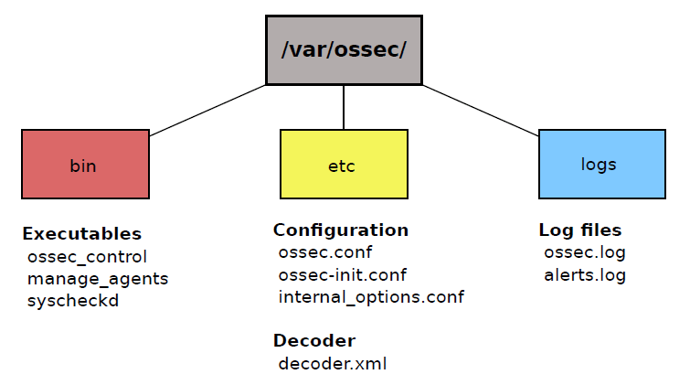
Figure 7.1 depicts OSSEC’s important directories and the corresponding files. The directories contain the binary files, configuration files, the decoder for decoding the events (see section 7.5) and the log files. They are all located in /var/ossec or in the directory which was specified during the installation, respectively.
Some of the essential executables are listed in this figure. For example ossec_control is used for starting the OSSEC system on the server or on an agent. syscheckd is the program for performing the file integrity check (section 7.1). To generate and import keys for the agents (see section 7.6) manage_agents is used.
All main configurations of OSSEC, for example setting the email notification, are done in ossec.conf. OSSEC’s meta-information that has been specified during the installation (see section 7.6) are stored in the ossec-init.conf and in internal_options.conf.
The file ossec.log stores everything that happens inside OSSEC. For example, if an OSSEC service starts or is canceled, this is listed in the ossec.log file. In alert.log all critical events are logged.
The OSSEC HIDS Analysis Process
When changes are made within the system, the type of this changing event has to be classified. Figure 7.2 shows the analysis process of such an event. It is performed in two major steps called predecoding and decoding. These steps extract relevant information from the event and rate its severity. This rating is done by finding a predefined rules which matches the event. The rule stores the severity of an event in different levels (0 to 15). If the event has been classified as an attack to the system, an alert is sent to the administrator and OSSEC tries to block the attack (active response). In the next sections, the steps predecoding and decoding are explained in more detail.

Predecoding
The predecoding step only extracts static information like time, date, hostname, program name and the log message. These are well-known fields of several used protocols. There are a lot of standards for computer data logging - like the Apple System Log (ASL) and syslog - which use a different formatting to handle and to store log messages. However, OSSEC is able to distinguish between these types of protocols. As an example, the following log message shows an invalid login of an unknown user using the ssh command (syslog standard).
Feb 27 13:11:18 master sshd[13030]: Invalid user evil from 136.172.13.56
OSSEC now extracts these information and classify the fields of this message. Table 7.1 shows the fields that are picked by the predecoding process and their description.

As mentioned before, there are several protocols that store log messages in different ways. The log messages have to be normalized so that the same rule can be applied for differently formatted log files. This is the task of the decoding phase that is described in the next section.
Decoding and Rule Matching
Following the predecoding phase, the decoding step extracts the nonstatic information of the events, e.g. the IP address, usernames and similar data, that can change from event to event. To get this data, a special XML file is used as a collection of predefined and user-defined decoders. They are matched with the current event using regular expressions. A decoder is specified by several options. These options define on which conditions a decoder will be executed. First of all, a decoder is delimited by a <decoder></decoder> tag, where the name of the decoder is specified. Within this tag all the possible options can be applied to fully refine the characteristics of the decoder. When working with syslog, the program name has to be set so that the decoder is only called if the program name appears in the log message. Another important option is the <prematch></prematch> tag. It can optionally be used jointly with the program name as an additional condition or as a single condition for non-syslog messages. To extract nonstatic information the decoder needs a <regex></regex> tag. This tag describes a regular expression which defines a pattern for matching the information included in the log message. As there are several fields in a message, the order of the fields also has to be specified, so that OSSEC knows how to parse out the fields of the message. This is done by the <order></order> tag.
Listing 7.1 gives an example of a decoder for an ssh event. It extracts the name and the source IP address of a user who tries to get access without any permissions via ssh corresponding to the given example.
- Listing 7.1 Example of a decoder for ssh.
<decoder name="ssh-invalid-user">
        <program_name>sshd</program_name>
        <prematch>^Invalid user</prematch>
        <regex> (\S+) from (\S+)$</regex>
        <order>user,srcip</order>
</decoder>
This decoder will only be called when the program name sshd has been extracted in the predecoding phase. Additionally, the prematch tag has to be satisfied. In this example the prematch option searches for the expression Invalid user in the log message. When this pattern will match what is in the log, the regular expression will be called to extract the user and source IP address. So only the decoder relevant for finding a rule associated with an invalid ssh success will be executed.
There are a lot of other options to specify the decoders. Here, the most important ones were explained. See OSSEC’s homepage[17] for more explanations on decoder options.
By now OSSEC has all the information it needs to find a rule that matches an event. Rules are typically stored as XML files in /var/ossec/rules. A rule is identified by a unique number and a severity level. Depending on this level, OSSEC decides if this event should be escalated to an alert.
Two types of rules exist: atomic and composite. Atomic rules are based on single events, whereas composite rules are related to multiple events. For example an ssh event can be escalated to an alert already after one single ssh authentication failure (atomic) or can be suspended until three authentications have failed (composite).
Setup and Configuration
Before starting the setup of OSSEC on the system, a C compiler and a makefile tool should be available on the system, because OSSEC is written in C and for compiling the sources, Makefiles are used. The sources of OSSEC are available at the OSSEC’s homepage and can simply be downloaded with the wget command (Listing 7.2).
- Listing 7.2 Getting the OSSEC source code.
wget http://www.ossec.net/files/ossec-hids-2.6.tar.gz
After extracting the archive, and changing to the extracted directory, the setup will start by executing the installer script install.sh (Listing 7.3). Subsequently, the user is guided through the setup.
- Listing 7.3 Extracting the archive and starting the installation.
tar -xvf ossec-hids-2.6.tar.gz
cd ossec-hids-2.6
./install.sh
OSSEC is a host-based intrusion detection system, that means if several computers are part of the cluster and all computers have to be monitored, OSSEC has to be installed on all of them. Furthermore, servers that manage all the data of the other computers - that means the agents - have to be declared. Depending on the intended type of usage of the computer (server or agent), OSSEC will be installed and configured in a different way. In the following, the setup of the server and the agents will be explained in separate sections. All installations were performed on Ubuntu Server 12.04.
Setup of the Server
The setup of the server is straight forward. One simply follows the instructions of the install script which include:
- setting the language (default is english)
- choosing Server as install type
- choosing the directory where OSSEC will be installed (default is /var/ossec)
- configuring the email notification (default is no email notification, see section 7.6.1 for how to set up the email notification)
- enabling/disabling the integrity check, the rootkit detection engine, active response and the firewall-drop response (enabled by default)
- adding IP addresses to the white list (localhost is the only IP address on the list by default)
- enabling/disabling remote syslog (allows redirecting the syslog messages from one host to another host)
When the setup is successful, the installer script provides some final information. If it was not successful, the script shows ”Building error. Unable to finish the installation” at the end of the compiler output. Maybe a prerequisite is missing; the OSSEC homepage might be a good help.
OSSEC is to be started with the command ossec-control located at the directory of OSSEC’s binary files (Listing 7.4). This command starts all the services as specified in the setup, e.g. rootkit detection and integrity check.
- Listing 7.4 Starting OSSEC.
/var/ossec/bin/ossec-control start
Whenever starting the server, OSSEC will be started automatically. OSSEC is active until the user stops it with ossec_control stop.
It recommended not to run any other intrusion detection systems in parallel with OSSEC. It is possible that they mutually influence each other. For example OSSEC could recognize the other intrusion detection and its actions as an “attack” to the system, when it modifies files that are monitored by OSSEC.
Email Notification
Some SMTP servers permit emails to be relayed from the host running the OSSEC HIDS. Because of that, it is better to install a local mail server. For this, all the settings are done on the OSSEC server. First a mail server is needed, for example postfix.[18] To process the emails, an email program has to be installed. The bsd-mailx, a command-line based email program is a possible choice for it (Listing 7.5).
- Listing 7.5 Installing the mail server and an email program.
sudo apt-get install postfix
sudo apt-get install bsd-mailx
Finally, OSSEC needs to know where to send the emails to. In the main configuration file ossec.conf, the following entry has to be added:
- Listing 7.6 Configuring the email notification in OSSEC.
<global>
   <email_notification>yes</email_notification>
   <email_to>root@master</email_to>
   <smtp_server>localhost</smtp_server>
   <email_from>ossec-notification</email_from>
</global>
This enables the email notification. All emails will be send to the user root who has an account on the localhost (the OSSEC server master in this example), where the mail server has been installed. The <email_from></email_from> tag specifies the sender of the email notification.
Subsequent to the base configuration, it is possible to personalize the email notification. At default, OSSEC will send an email for every alert. This can be customized by setting the email alert level. Events are rated by their severity ranging from 0 to 15. Listing 7.7 shows how to set the email alert level, that means the minimum level an event must have so that an email will be sent. In the above example (Listing 7.6) there will only be sent an email if the event has an severity level greater than 7. The same option can be specified for writing the log files. In the below example (Listing 7.7) every event will be logged and saved in a log file, because the log alert level is set on the smallest possible severity level 0. Both options are located in the <alert></alert> tag in the main configuration file ossec.conf.
- Listing 7.7 Setting the email alert level.
<alerts>
   <log_alert_level>0</log_alert_level>
   <email_alert_level>7</email_alert_level>
</alerts>
Setup of the Agent
Before installing the agents, the server needs to know the agents from which it has to collect the data. The agents must be able to identify themselves to the server and the server must be able to validate the identity of an agent.
The communication between server and agent is handled by key management. Keys are generated on the server and are then imported on each agent. OSSEC offers a tool, to perform the key management: manage_agents (Listing 7.8). First this tool has to be executed on the server to add the agents.
- Listing 7.8 Starting the key management.
/var/ossec/bin/manage_agents
After starting the tool, there are five options to choose:
- (A)
- for adding an agent
- (E)
- for extracting the key for an agent
- (L)
- for listing already added agents
- (R)
- for removing an agent and
- (Q)
- to quit the service
When adding an agent (option (A)), the user is prompted for host details and identifier for the agent. This includes a name, the IP address of the agent and a unique identifier which is a three-digit number (Listing 7.9]).
- Listing 7.9 Adding an agent.
- Adding a new agent (use '\q' to return to the main menu).
 Please provide the following:
 * A name for the new agent: worker1
 * The IP address of the new agent: 10.0.0.1
 * An ID for the new agent[001]: 001
Agent information:
 ID: 001
 Name: worker1
 IP Address: 10.0.0.1
Confirm adding it? (y/n): y
Agent added.
Then OSSEC has to be installed on each agent separately using the installer script. The setup is very similar to the setup of the server (see section 7.6.1), the only difference is that the agents need to know the IP address of the server (Listing 7.10). Here the server’s IP address in the subnetwork is needed (Hint: ifconfig eth1).
- Listing 7.10 Setup of OSSEC on the agent’s side. The only difference is the setting of the server’s IP address.
3 - Configuring the OSSEC HIDS.
   3.1 - What's the IP Address of the OSSEC HIDS server?: 10.0.0.250
       - Adding Server IP 10.0.0.250
After the installation has finished, a key for each agent has to be generated. This is done by starting the manage_agents tool again on the server’s side and then choosing option (E) for extracting a key for the agent. By selecting an agent by its three-digit identification number, a key will be generated (Listing 7.11). This key can be copied to the clipboard.
- Listing 7.11 Generating the key for an agent (worker1).
Available agents:
   ID: 001, Name: worker1, IP: 10.0.0.1
Provide the ID of the agent to extract the key: 001
Agent key information for '001' is:
   MDAxIG1hcnMgMTkyLjE2OC42NS40MCBmY2UzMjM4OT
   c1ODgzYTU4ZWM3YTRkYWJiZTJmMjQ2Y2ViODhmMzlm
   YjE3MmI4OGUzMTE0MDczMzVhYjk2OTRh
Press ENTER to return to the main menu.
To import the key, the manage_agents tool has to be executed on the corresponding agent. There are only two options to choose: (I) for importing a key from the server and (Q) to quit the service. After choosing the option (I), the key value is pasted from the clipboard into the terminal behind the prompt Paste it here. The tool provides some information about the agent for verifying the agent.
- Listing 7.12 Importing the key of the agent (worker1) generated on the server.
Paste it here:
   MDAxIG1hcnMgMTkyLjE2OC42NS40MCBmY2UzMjM4OT
   c1ODgzYTU4ZWM3YTRkYWJiZTJmMjQ2Y2ViODhmMzlm
   YjE3MmI4OGUzMTE0MDczMzVhYjk2OTRh
Agent information:
   ID:001
   Name:worker1
   IP Address:10.0.0.1
   Confirm adding it?(y/n): y
Added.
Then the service is quitted and OSSEC is restarted with ossec_control restart. When the restart and the connection to the server are successful, you can find a similar entry - seen in Listing 7.13 - in the log file ossec.log of the agent.
- Listing 7.13 Success of the setup of the agent.
2007/10/10 23:25:48 ossec-agentd: Connecting to server (<IP-address-server>:1514).
2007/10/10 23:25:48 ossec-agentd(4102): Connected to the server.
The OSSEC Web User Interface
The web user interface (WUI) visualizes all the statistics that are collected during the running time of OSSEC. This includes the events, alerts, statistics about firewall drops and log file entries in a tabular form. OSSEC’s web-based interface makes the access to the statistics more comfortable.
The following sections show how to setup the WUI on an OSSEC HIDS server and the main functionality of the WUI.
Setup
The WUI runs on a fixed OSSEC HIDS server which collects and manages the agent’s data. The WUI cannot be installed on an agent, because all collected alerts are sent back to an OSSEC HIDS server for further processing. Before installing the WUI, there are some basic prerequisites that have to be met. The OSSEC HIDS server needs to be set as an HTTP web server - choosing apache2 here - and a package including the interpreter for the server-side scripting language PHP has to be installed (Listing 7.14). With this, the code containing the web page with php code can be interpreted by the web server.
- Listing 7.14 Installing the apache server and php5.
sudo apt-get install apache2 php5
After downloading and extracting the archive containing the sources (Listing 7.15), the extracted directory is moved to /var/www, so as the web server can access the files.
- Listing 7.15 Getting the WUI sources.
wget http://www.ossec.net/files/ossec-wui-0.3.tar.gz
tar -xvf http://www.ossec.net/files/ossec-wui-0.3.tar.gz
The directory contains a installer script guiding the user through the setup (Listing 7.16).
- Listing 7.16 Extracting the wui files, moving it to /var/www and starting the setup.
mv ossec-wui-0.3 /var/www
cd /var/www/ossec-wui-0.3
./setup.sh
The installation prompts for a username and a password (Listing 7.17). After this, the installation starts and the installer reports whether the setup was successful.
- Listing 7.17 Installing the WUI.
Setting up ossec ui...
Username: schroeder
New password:
Re-type new password:
Adding password for user schroeder
...#Setup output
Setup completed successfully.
To complete the setup, the web server user has to be added to the ossec group (Listing 7.18). This user is typically apache, www or www-data.
- Listing 7.18 Adding user www-data to ossec group.
adduser www-data ossec
After restarting the whole system, the WUI is available at http://<ip-address-of-webserver>/ossec-wui-0.3/.
Functionality
The WUI offers a powerful functionality that helps the user to view the events that are happening within the system. Figure [fig:overview] shows the main window. It gives an overview about the available server(s) and agents, the latest modified files and the latest events. The available agents are described by their name and the associated IP address. This information is shown when clicking on the corresponding agent. If the agent is inactive or unable to connect to the server, the word Inactive is displayed beside the agent’s name. In the figure, the agent named worker1 is currently set inactive. Only the OSSEC server is available.

Moreover the main window contains four tabs, where each of them provides a specific functionality. These are
- Main, shows the main window
- Search, allows searching through collected alerts
- Integrity Checking, allows searching through collected syscheck alerts and
- Stats, shows aggregated statistics about collected alerts.
The fifth tab About does not provide a special service and just shows information about the WUI version and its contributors.
The search window (Figure 7.4) offers a query interface with a lot of possible options to specify the kind of alerts the user is searching for. Options of interest may be the minimum severity level of an alert, the category (e.g authentication control) and the log formats (e.g sshd). A specific search period can be set. Alternatively, by choosing the real time monitoring, the WUI shows all the upcoming events.
There are some more options to reduce the search results. A rule ID can be specified, so that only alerts and events are shown that are allocated to this rule number. The field Pattern searches for a pattern in an event described by regular expressions. To show only events from a particular agent (for example worker1) or from an user account (for example root), the fields Location and User are used. When there are too many search results, the maximal number of alerts to display can be restricted with the field Max Alerts.
When results are found, the WUI divides the types of alerts into three classes:
- Severity breakdown
- Alerts are sorted by their severity level
- Rules breakdown
- Informs about the alert’s corresponding rule ID
- Src IP breakdown
- Informs about the alert’s corresponding source ID, i.e. the user who triggered this alert.

The WUI also shows files that have been modified on the server and on all agents. Clicking on a specific file, for example /etc/resolv.conf in Figure 7.5, gives further information about where the file is located - specified by the server’s or agent’s name and a directory path - and when it has been modified.

Figure 7.6 shows a detailed view of modified files for a particular agent. This view can be selected by choosing an agent via the drop down menu offering all the agents that are part of the OSSEC system. Clicking Dump database gives the overview of all files that have changed for this agent.

Figure 7.7 shows the statistics of a selected date. It shows values aggregated over all agents sorted by severity level of events and by rules (described by their rule ID), respectively. Moreover it counts the total and the averaged number of events and how many events are classified as alerts.

An event is represented as in Figure 7.8. This representation is used in the main window and when showing the search results. It contains the following information: The date and time when the OSSEC agent has recognized the event are shown. The date and time stamps are displayed at the beginning of every event. The rule ID (Rule Id) that is associated with the event has a link to pieces of information about the rule. Clicking on it will redirect the user to the web page containing rule specific information. The severity level of an event is also shown in this representation (level). The Location field gives information on the agent that reported the event and what file is associated with the event. Description summarizes the event in a short description.

Summary
In this chapter OSSEC was introduced. OSSEC is meant to be a powerful tool to monitor a computer cluster. It includes features as file integrity checking, log monitoring, active response for blocking attacks and rootkit detection. OSSEC uses a special analysis to inspect log files. Log messages are processed in two steps. First the predecoding (section 7.5.1) was presented and then the decoding step (section 7.5.2) was explained. In the decoding step, an XML file is used to extract specific information from events.
The setup of OSSEC was explained in two parts, the server installation (section 7.6.1) and the agent installation (section 7.6.2). For the agent installation it was important to generate keys to make the communication between server and agents possible. The server installation included the configuration of a local email notification (section 7.6.1). This was necessary, because many SMTP servers do not accept messages that have been sent from the OSSEC server.
OSSEC offers an optional feature: the web user interface. Its installation - including the configuration of the OSSEC server as an apache web server - and functionality were explained in section [sec:wui].
The OSSEC basic configuration with all its rules and decoders actually offers a useful detection of well-known events that can occur in a system. However, it is possible to refine OSSEC’s functionality with self-defined rules. This was not described here, because it would go beyond the scope of this report. For further studies it would be interesting to adjust OSSEC’s functionality to the characteristics of the current computer cluster by defining own rules. For this, one has to analyze events that typically occur in the actual computer cluster. The main aim is to create useful and appropriate decoders and rules.
Munin
Installation of the software Munin
Munin is a software system based on Linux. It measures the server load. This requires a 64-bit computer!
First unzip and to install the software package Munin using the command “sudo apt-get install munin munin-node”. This extracts the entire Munin software package on the Linux operating system. Once you’ve performed this, enter sudo nano /etc/munin/munin.conf to open the configuration menu. The file should look like this:
#htmldir /var/www/statistics
#logdir/var/log/munin
#rundir/var/run/munin
You delete the comments by removing the # character from the commands so that the program can read and execute it. After you installed the munin plugins with sudo nano /usr/share/munin/plugins. The program will then restart with sudo /etc/init.d/munin-node restart, so that it accepts all new settings. The command sudo apt-get install apache2
installs the web server and
sudo/etc/apache2/mods-available/status/conf
shows finally the configuration menu. Here the extended status must be set to On to run Munin as desired. The sudo a2enmod status needs to be activated. This must be on enabeld.
After that the plug-ins are going to be enabled. For this one must enter the following commands in the command line:
sudo ln-s/urs/share/munin/plugins/ _apache/etc/munin/plugins ln-s/urs/share/munin/plugins/ apache_proccess/etc/ munin/plugins
ln-s/urs/share/munin/plugins/_volume/etc/munin/ plugins
To change the settings of Munin you restart the system with:
sudo /etc/init.d/apache2 restart
The following command installs the graphic package:
sudo apt-get install libwww-perl
This is required for the design of the graphs.
Working with Munin
The software system Munin must be connected to an Internet server so that its visual interface can be displayed. For this purpose, again, open the configuration file with this command:
sudo nano /etc/munin/munin.conf
The shown IP Name localdomain for locally called internet domain domain will be changed to the name Master. The displayed IP address must be in the master has be changed to 127.0.0.1.Worker gets the number 10.0.2.2. ( Each working group got different IP extensions, here the 2.2).
## First our “normal” host. [server02/ Master] address 127.0.0.1
(Vgl. http://help.ubuntu-se.org/9.10/serverguide/sv/munin.html)
On a Windows computer always the same name must be used. When the web browsers can not open Munin, the name must be changed in the sudo/etc/hosts file. Subsequently, enter the IP from the Master/munin in the internet browser and trie to open the Munin page or the software system. If the installation was successful, Munin can be accessed and measures the server load. However, the measurement takes some time to complete because Munin measures per day/month/year or different workloads on a few servers. It displays the minimum and maximum values (see on the next page the picture of the software system Munin). In addition, the system measures at different times. Updates for Munin appear and also get reported by the program. It is also displayed when the server is can not be reached, for example, during a power failure or computer crash.

(Quelle: http://zockertown.de/s9y/index.php?/archives/1426-Munin-ist-schon-toll.html)
The advantage of the program is that you can react to a failure of a server even with a large number of servers and quickly detect which server is down. This must then be optionally repaired or renewed.
Example of computer cluster in Munin, vgl. http://munin.ping.uio.no/
Overview • ping.uio.no
o aquarius.ping.uio.no [ disk exim network processes system ]
o bache.ping.uio.no [ disk network nfs
postfix processes system time ]
o bambi.ping.uio.no [ disk network nfs
processes system time ]
o bimbo.ping.uio.no [ disk exim network nfs
other processes system ]
o bottolf.ping.uio.no [ disk exim network
nfs processes system time ]
o cirrus.ping.uio.no [ disk exim network
processes sensors system ]
o cumulus.ping.uio.no [ disk exim network
processes sensors system ]
o freddy.ping.uio.no [ disk network nfs
postfix processes sensors system time ]
o galactica.ping.uio.no [ disk exim
network nfs postfix printing processes
system ]
o gud.ping.uio.no [ disk network nfs
postfix printing processes sensors
system ]
o kjell.ping.uio.no [ disk network
nfs postfix processes sensors system time ]
o knuth.ping.uio.no [ apache disk mysql
network nfs postfix processes sensors system time ]
o m.ping.uio.no [ disk exim network nfs
printing processes sensors system ]
o matz.ping.uio.no [ disk network nfs
processes system ]
o meg.ping.uio.no [ disk network nfs other processes system ]
o pike.ping.uio.no [ apache disk exim
munin network printing processes sensors
system time virtual machines ]
o ponnypetra.ping.uio.no [ disk network other processes system ]
o rosa.ping.uio.no [ disk network nfs
processes system time ]
o rossum.ping.uio.no [ apache disk exim network nfs other processes system time ]
o tetra.ping.uio.no [ disk network
processes system ]
o urias.ping.uio.no [ disk network nfs other processes system time ]
o utslett.ping.uio.no [ disk munin
network processes system ]
On the picture you can see the individual process servers and systems. In Ubuntu all packets have a start and stop function. These control the services.
Therefore one must enter: sudo /etc/init.d/munin-nodestart|stop|restart|force-reload|try-restart
“Restart” restarts the system, existing systems on the server will be stopped. “Try -restart restarts the service when he was stopped before.”
Warnings
If the limits of the capacity utilization in the Munin server are exceeded, these values are usually displayed in red. One can send then alerts via e-mail, so that the maximum disk space is not exceeded. For this purpose, open the file munin.conf ( wiki.ubuntuusers.de/Munin). These commands are then added:
# Drop somejuser@fnord.comm and antoherurser@blibb.com an email
everytime
# something changes ( OK Warning, CRITICAL OK, etc)
Contacts me
Contacts.me.command mail -s “Munin notification ( var:host)” user@example.com
Contact.me.always_send warning critical
The email address must be adapted to your own system. This should be done even the utilization values are determined from when the server threatens to overflow, to timely send a warning to the user can. Before a postfix should be installed and configured so that the e-mails are sent to all users. For each host, this can be achieved as follows (see example from the configuration file of Munin.):
(localhost.localdomain/Master)
Address 127.0.0.1.
use_node_name yes
<plugin>.<fieldname>. (critical,warning) <value>
The plugin is accessed via the URL of the graph. The field name can be copied from the Munin graph. Under Internal name is the fieldname shown. Critical warning can be freely selected. The value is determined as described above and upon reaching/exceeding a warning e-mail sent to all users.
Example of a Server Warning entry in Munin
“[localhost.localdomain]
address 127.0.0.1
use_node_name yes
fd._dev_evms_hda2.warning 70
df._dev_evms_hda2.critical 95
df._dev_mapper_hda5.warning 70
df._dev_mapper_hda5.critical 70”
Here was 70 determined as a critical value and 95 selected to be a very critical value. The values should be carefully selected and not too low, because the user gets an warning email and can be frightened. The warnings should also be sent in any case with the truly critical values, so you can, if necessary, load the system with a backup.
CPU main processor
Munin can also measure the load on the main processor. This is a central processing unit executing a program. This also works for central host computers, connected to the plurality of terminals. Even earlier computer server performance and data can be compared with one another with Munin. The master collects the performance data, the node stores them and generates a graphic on the Web interface. The storage of the graphic is made via the RRDtool.

Munin errors and cleanup
Various types of errors can occur, for example, the IP address may change from one day to the other. Munin can not achieve the desired browser page therefore. In this case, the address in the configuration file needs adjustment. It is not so easy to change the name of the localdomainserver.
White bars in the graphic:
The cause may be that the user has configured a graphic file or a mistake when while unpacking the package. When installing the permissions mistakes can happen easily, because then e.g. no warning e-mails can be sent when the server overflows.
SnortIDS
What is Snort?
Snort is a network intrusion detection system and a network intrusion prevention system. It is a free and open source system created by Martin Roesch in 1998. Snort was developed by Sourcefire and in 2009, Snort entered InfoWorld’s Open Source Hall of Fame as one of the “greatest open source software of all time“.
Usage
Snort has the the ability to perform real-time traffic analysis and packet logging on Internet Protocol networks and performs protocol analysis, content searching, and content matching. Snort can also be used to detect probes or attacks, including operating system fingerprinting attempts, common gateway interface, buffer overflows, server message block probes and stealth port scans.
Snort has three main configuration modes: sniffer, packet logger and network intrusion detection. In sniffer mode, Snort will read the network packets and display them on the console. Snort will log packets to the disk in the packet logger mode and in the intrusion detection mode, Snort will monitor the network traffic and analyze it against a rule set the user has defined. Snort will then alarm the user or it will perform a specific action based on what has happened.
Packages
LAMP-Server
LAMP is a combination of free, open source software, LAMP refers to Linux, Apache HTTP Server, MySQL and PHP, Perl or Python. The exact Software may vary in the LAMP-Package and it is not designed by its original authors as one Package. But it is developed in close conjunction, therefore it is easy adaptable. When used together, they support web application servers.
BASE
BASE is the Basic Analysis and Security Engine. It is based on the code from the Analysis Console for Intrusion Databases (ACID) project. This application provides a web front-end to query and analyze the alerts coming from a SNORT IDS system.
BASE is a web interface to perform analysis of intrusions that snort has detected on your network. It uses a user authentication and role-base system, so that you as the security admin can decide what and how much information each user can see. It also has a simple to use, web-based setup program for people not comfortable with editing files directly.
Setup
For SnortIDS you will use the LAMP Server. It will serve as a HTTP server for ACID, your Webinterface, and will also serve as a MySQL backend for Snort. Ubuntu 12.04 LTS was used for this Setup.
LAMP-Server
root@master:/# sudo tasksel install lamp-server
tasksel: Starts a simple Interface for the user to select general tasks for the installation.
You will be prompted to select a MySQL root password. This will be needed further in the installation.
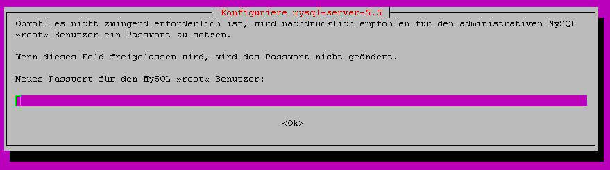
Snort-Mysql
First you create a database.
root@master:/# mysql -u root -p
mysql> create database snort;
mysql> GRANT SELECT, INSERT, UPDATE, DELETE, CREATE, DROP, INDEX, ALTER, CREATE TEMPORARY TABLES, LOCK TABLES ON snort.* TO 'masterusername'@'localhost' IDENTIFIED BY 'password';
mysql> FLUSH PRIVILEGES;
mysql> quit
root@master:/# _
Further on you can now install SNORT
root@master:/# sudo apt-get -y install snort-mysql
You will be prompted to enter the IP address for your local network. It is your cluster-network, that you want to protect. The Classless Inter-Domain Routing (CIDR) format have to be used. 10.0.x.0/24

You will be asked, if you wish to set up a database for use with Snort.

Choose no. You already created the database, you only need to configure it. With this you will update the Snort table structure.
root@master:/# pushd /usr/share/doc/snort-mysql
root@master:/# sudo zcat create_mysql.gz | mysql -u snort -p snort
- The syntax is: mysql -u <username> -p <prompt for password> <database>
root@master:/# popd
Now modify the Snort configuration file to include your MySQL specific information.
root@master:/# sudo sed -i "s/output\ log_tcpdump:\ tcpdump.log/#output\ log_tcpdump:\ tcpdump.log\noutput\ database:\ log,\ mysql, user=snort password=password dbname=snort host=localhost/" /etc/snort/snort.conf
The above line was located at line number 786 /etc/snort/snort.conf. The snippet simply places a comment in front of the output for the log, and appends the output line for our database.
Now remove the pending Snort database configuration file.
root@master:/# sudo rm -rf /etc/snort/db-pending-config
Start Snort.
root@master:/# sudo /etc/init.d/snort start
To check the status of the Snort daemons use:
root@master:/# sudo /etc/init.d/snort status
Acidbase
To check the output of Snort, you will use ACID, a web front-end.
root@master:/# sudo apt-get -y install acidbase
You will be asked to configure a database for acidbase. Choose yes and use MySQL.

You will be prompted for the password of the database administrator. This is the same password you used when MySQL was initially installed with LAMP.
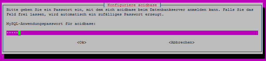
To get access for the acidbase web front-end, you have to edit the apache.conf
root@master:/# sudo sed -i "s#allow\ from\ 127.0.0.0/255.0.0.0#allow\ from\ 127.0.0.0/255.0.0.0\ 'your IP'/255.255.255.0#" /etc/acidbase/apache.conf
This will allow your and the machine to get access to the front-end.
You can also allow access for all

To take affect, you have to restart apache.
root@master:/# sudo /etc/init.d/apache2 restart
Browse to: http://’IP of the machine with SNORT’/acidbase
For testing purpose perform a portscan of the Snort host. You will need the nmap-package for this.
root@master:/# sudo nmap -p1-65535 -sV -sS -O 'IP of your SNORT-machine'
If something is not working properly, try to reconfigure SNORT. With the following command, you can reset the IP´s.
root@master:/# sudo dpkg-reconfigure snort-mysql
Prelude
Prelude is a sensor-based monitoring system that is a perfect choice for monitoring a cluster because of it’s the manager module. This guide explains what Prelude is and how you install it in a virtual Ubuntu system.
What is Prelude?
Prelude is a so-called ’Intrusion Detection System’ (IDS). A distinction is made between ’host’- and ’network’-based intrusion detection systems. A HIDS protects and controls the activities directly on the operating system, it takes care of the logging and kernel files and to the registry. A NIDS on the other hand takes care of the network monitoring system employed. Prelude combines these two methods, and thus belongs to the group of “Hybrid Intrusion Detection System”.
Manager
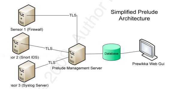
The Prelude-Manager is the heart of the software, here all messages of the sensors come together and then are written into the database. The sensors can observe very different places such as various logs, or the kernel itself. In this way, a sensor is arranged for each relevant interface, which then being conntected to the manager. The manager collects, sorts and normalizes the incoming data and stores it in IDMEF format in the created database.
In addition to the sensors Prelude brings from home, it is also possible to register third-party sensors to the Manager.

Software Packages
So Prelude is runs smoothly, it is necessary to install a handful of packages on your system.
- prelude-manager: The Prelude Manager is, as already described, the heart of the software. This is where all messages from the sensors come together.
- prelude-lml: The Prelude Log Monitoring Lackey reads various log files and provides them as input for the manager. In our case, we later read from the auth.log file, this gives us information on the login attempts in our system.
- prewikka: Prewikka graphically prepares our data that the manager has written to the database, so that we can also recall it from the browser.
- apache2: An Apache Webserver is necessary for us to open the site Prewikka provides.
- postgresql-9.1: We need a total of two databases, in this case it is advisable to use PostgreSQl instead of mySQL, more on that later. The manager and Prewikka each require their own database.
Installation
Shell commands can be recognized by the following scheme:
# nano /etc/hosts
Requirements
This installation has been tested on a virtual system with one master and several workers. On all machines the 64 bit version of Ubuntu Server was used. For ease of passage of the installation, it is recommended to give appropriate “root” rights once with the command
# sudo su
.
Step by Step Installation
- Step 1
-
Install all software packages: (All packets are solely installed on the master)
# apt-get install prelude-lml prelude-manager prelude-correlator prelude-notify apache2 postgresql-9.1 prewikka
The user is eventually asked if he wants to set up the database using a wizard, this is recommended here for inexperienced users. - Step 2
-
Now various configuration files must be set. We start with the Prelude configuration.
# nano /etc/prelude/default/global.conf
 Figure 10.3: IMPORTANT [NODE-ADDRESS] must be commented.
Here, the “node-name” must be entered, as well as the right address. When on a virtual machine, use the following address for the local environment “127.0.0.1”. It is important that [NODE ADDRESS] is also commented here!
- Step 3
-
Start the Prelude Manager:
# /etc/init.d/prelude-manager start
Here we are told that the prelude-manager has yet to be activated. The matching file is given in the error message.
prelude-manager disabled, please adjust the configuration to your needs * and then set RUN to ’yes’ in /etc/default/prelude-manager to enable it.
After activating the Prelude Manager in the following file, we start it again with the command from above.
# nano /etc/default/prelude-manager
- Step 4
-
The Prelude sensors must be registered in the manager, so that they can communicate with each other. For this we register the Prelude in this step - LML Sensor to the Manager. On the Manager, we run the following command to register the prelude-lml sensor.
# prelude-admin register prelude-lml ’idmef:w admin:r’ 127.0.0.1 –uid 0 –gid 0
 Figure 10.4: The manager now waits for the password
This now awaits the entry of a on the server generated password. Since our Prelude-lml tool is running on the same master as the manager, a second terminal window should be used.
# prelude-admin registration-server prelude-manager
 Figure 10.5: The by the sensor generated password must now be entered in the manager
This command generates for our sensor a password, which is necessary to enter at the registration, after successfully entering the password in the manager, the registration must again be confirmed. Now Manager and Sensor (Prelude-lml) are connected to each other.
 Figure 10.6: Registration successful!
- Step 5
-
We configured our managers already in step 2, now the sensor (Prelude-lml) must be set. For this, we edit the file:
# nano /etc/prelude-lml/prelude-lml.conf
Here are two lines need to be commented, so that the sensor has set the correct server address.
[prelude]
server-addr = 127.0.0.1
- Step 6
-
Prelude is now fully functional, but we still lack the graphical representation of the results, we get this with Prewikka displayed in the browser. Therefore it is recommended once again to check the databases.
# nano /etc/prewikka/prewikka.conf- Listing 10.1 Database name and user (example)
type: pgsqlhost: localhost user: prelude pass: prelude name: prelude [database] type: pgsql host: localhost user: prewikka pass: prewikka name: prewikka - Step 7
-
Lastly the Apache server can be configured so that it also takes the necessary files from Prewikka.
# nano /etc/apache2/apache2.conf
At the end of this file, the following code must be added:- Listing 10.2 Apache configuration for Prewikka
Alias /prewikka/prewikka/ /usr/share/prewikka/htdocs/
ScriptAlias /prewikka/ /usr/share/prewikka/cgi-bin/prewikka.cgi
<Directory /usr/share/prewikka/htdocs/>
Options None AllowOverride None Order allow,deny Allow from all</Directory> <Directory /usr/share/prewikka/cgi-bin/>
AllowOverride None Options ExecCGI <IfModule mod_mime.c> AddHandler cgi-script .cgi </IfModule> Order allow,deny Allow from all</Directory>
Apache has to be restarted once after reconfiguration.
# /etc/init.d/apache2 restart
- Step 8
-
Prewikka must be started (after every reboot) with the following daemon:
# /usr/bin/prewikka-httpd
- Step 9
-
Now Prewikka can be accessed in the browser. (Of course, replace the IP adress with your eth0 inet adress)
192.168.178.56/prewikka/
Name: admin
Password: admin
Issues during installation
When you install a few problems might occur, a few of them, I would like to briefly discuss.
lack of access rights in step 8
eventually an error that reports a lack of privileges of prewikka.conf file appears when starting Prewikka in step 8. If this error occurs the rights to the file must be again be adjusted with the command, .
# chmod 755 /etc/prewikka/prewikka.conf
PreSQL instead of mySQL
The reason we use PreSQL and not mySQL is that Prelude uses outdated database settings. It uses the outdated command ’TYPE = InnoDB’, however, mySQL 5.0+ accepts only the command ENGINE = InnoDB ’. This can indeed be corrected in the file:
# nano /usr/share/libpreludedb/classic/mysql.sql
It then accepts this file also, but then fails to start from the prelude-manager due to an error in the libpreludedb.
It is therefore advisable to use a PreSQL database for Prelude.
Prewikka
We use Prewikka so that our data, the Prelude Manager collects from all its sensors, are clearly displayed in a graphical web interface. Here we get all the needed information that can also be found in the Prelude Manager database. In our case, we have only registered the Prelude Manager and the Prelude-LML sensor, which currently reads the auth.log file of the system.
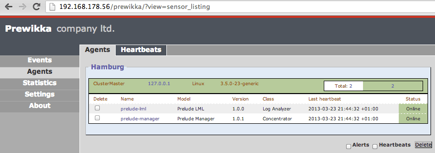

Useful websites
- Prelude website: https://www.prelude-ids.org/
- Prelude Manager Guide: https://www.prelude-ids.org/wiki/1/PreludeManager
- Prewikka Guide: http://security.ncsa.illinois.edu/research/mithril/PrewikkaInstall.html
- PostgreSQL Guide: https://help.ubuntu.com/community/PostgreSQL
- Video Install Tutorial: http://www.youtube.com/watch?v=oV4JCqi0FJw
Firestarter
What is Firestarter?
Firestarter is a firewall in Linux, which protects against viruses. “It is merely a graphical front-end for creating iptable rules and for displaying information on the network interface ”(see http://wiki.ubuntuusers.de/Firestarter).
Firestarter is intended only as a “surface”. “It reaches deep into the system and should be run as a tray in the background.”
Installation of Firestarter
With
sudo apt-get install firestarter
you install the firewall Firestarter. The command
sudo gksu gedit /etc/firestarter/user-pre
installs in addition the interface. Furthermore
sudo /etc/init.d/firestarter restart
restarts the system, so the installation can be completed.
Applications -> Internet -> Firestarter
activates opens the Firestarter gui. Then the Firestarter settings will be adapted using a Setup menu.
Adaption of Firestarter
Step 1:
- Network device setup
For this one must make the following settings:
- Set detected device ethernet to eth1
- IP Adress is assigned via DHCP checkmark
- click forward
Step 2
- Ready to start your firewall
- Start firewall now, restart system
- click save, Firestarter should start now
Step 3
Internet connection sharing setup
- internet connection sharing setup menu
- internet connection sharing setup
- change to IP tunnel
- click DHCP Server details
- forward
(Example of https://help.ubuntu.com/community/Firestarter)
VPN-Connection
When the PC is only connected through a VPM to the Internet, you have to enter:
Example of: Allowing a VPN connection (replace xxx.xxx.xxx.xxx by a IP address of the VPN server)
/sbin/iptables -A INPUT -j ACCEPT -s xxx.xxx.xxx.xxx -p esp
/sbin/iptables -A INPUT -j ACCEPT -s xxx.xxx.xxx.xxx -p udp -m multiport –sports isakmp,10000
/sbin/iptables -A INPUT -j ACCEPT -i tun+
/sbin/iptables -A OUTPUT -j ACCEPT -d xxx.xxx.xxx.xxx -p esp
/sbin/iptables -A OUTPUT -j ACCEPT -d xxx.xxx.xxx.xxx -p udp -m multiport –dports isakmp,10000
/sbin/iptables -A OUTPUT -j ACCEPT -o tun+

Lock Firewall locks the firewall.
Stop Firewall stops the firewall
Network displays the current activities of the various network servers.
The firewall should start when calling the system to protect the program.
Eth0 is the network card of the system that is connected to the local Internet.
The textbf Help function provides various help information to assist with standard issues. These have occurred as often. This is a FAQ that has listed the common error and their aids. The user can then look to see if he can solve the problem. The wiki forums are also a good help to find codes that one does not know or to get help with specific problems.
Simplicity of Use
Firestarter is quite easy to install, but a very complex security system. You can define which connection attempts should be blocked on the log, useful for known viruses or websites. There is a central hub where you manage inbound and outbound rules. It does not need to be used on a desktop system, due in Linux no services are provided to the outside
(see http://www.tecchannel.de/produkte/sicherheit/desktop-firewalls/
firestarter/test/). An almost easy to install system because the system takes a user through the installation.
Firestarter Errors and Cleanup
With Firestarter a problem is that the firewall is engaged too deeply into the operating system. Linux is not quite so often attacked as Windows, because of the underlying infrastructure of the system. A firewall should be installed yet. The packets of each software require a very large number of MB and requires corresponding time before the system unpacked it. The VPN configuration is somewhat complicated for the user. It requires appropriate exercise time until you get familiar with the system. The codes are initially easily mistyped in the beginning, if you are not so familiar. The firewall should start when booting the system to protect it accordingly.
Torque
Torque is an open source resource manager based on the original PBS project (http://www.pbsworks.com/). It is responsible to start, delete or to monitor jobs and thus supports a scheduler that could not manage the jobs without these functions otherwise. Therefore Torque brings it its own scheduler (pbs_sched), but you can also use other. Torque is flexible enough to perform space planning, but is used mostly in clusters. How to install and configure Torque for simple jobs on a cluster is described below. To install the latest version of Torque, you should not use the package from Ubuntu, but the package from the following website: http://www.adaptivecomputing.com/products/open-source/torque/.
Download Torque
Download the files in the master (here we used version 4.1.4).
$ sudo wget http://adaptive.wpengine.com/resources/downloads/torque/torque-4.1.4.tar.gz
Unzip file and navigate to the directory
$ tar -xzvf torque-4.1.4.tar.gz
$ cd torque-4.1.4/
When configuring and installing one remains best in this directory.
Configure and install the package on the master
Set Directory
By default make install installs all files in in /usr/local/bin, /usr/local/lib, /usr/local/sbin, /usr/local/include, and /usr/local/man.
You can also specify a different folder where the files should be stored by putting -–prefix=$directoryname behind ./configure. So If you don’t want to change anything, you do not need to consider this step.
Set Library Folder
Create a new file: /etc/ld.so.conf.d/torque.conf
$ sudo nano /etc/ld.so.conf.d/torque.conf
There you write the path to the libraries. In the standard setting, it would be /usr/local/lib (is home defined as a directory it would be /home/lib). Then enter the following command:
$ sudo ldconfig
Perform Configure
To execute configure you have to install build-essentials, libssl-devel and libxml2-devel with this command:
$ sudo apt-get install build-essentials libssl-dev libxml2-dev
If you excute ./configure you will get an error that libxml2-devel isn’t installed. This is a bug in Torque and can be fixed with following steps:
Firstly two lines in the configure.ac file need to be changed (see screenshot).
$ sudo nano configure.ac

The minus describes the line that needs to be changed, the plus describes how the line should read after the change. It is best to look for a keyword for the line to be changed because the file has a lot of lines.
After that execute autoconf:
$ sudo autoconf
and change the configure file:
sudo nano configure

Again, you look for the yellow marked line and change in the end (red rectangle) the -1 in a -l.
Now you can run ./configure and it should finish without errors.
sudo ./configure
In the end also run make and make install.
sudo make
sudo make install
By default, make install creates the directory /var/spool/torque. This directory is referred to as TORQUE_HOME. There, various subfolders are created that are used to configure and run the program.
Install Torque on the Nodes
Create packages
Torque has the function to create the packages, which uses the configurations and then can be installed on the nodes. Use the command make for this.
make packages
The packages are stored in the torque-4.1.4/ and must be copied from there in a shared directory the nodes have access to. In our case it would be the /home directory.
For example:
cp torque-package-mom-linux-i686.sh /home
On the nodes only the mom-linux package is needed. All others are optional.
Install Package
On the node you navigate to the directory in which you have copied the package and install it with the following command:
./torque-package-mom-linux-i686.sh –install
Torque Konfigurieren
Initialise serverdb
In the directory TORQUE_HOME/server_priv are configurations and information located that the pbs_server Service uses. To initialise the file serverdb run following command:
sudo ./torque.setup
Then the pbs_server needs a restart.
sudo qterm
sudo pbs_server
The server properties can be see by the following command:
sudo qmgr -c ’p s’
Specify Nodes
Thus, the pbs_server recognizes which computers in the network are the nodes. For this create in the directory TORQUE_HOME/server_priv a new file nodes:
sudo nano nodes
In this file, the nodes will be stored with their name. Normally it is sufficient to write the names in the file, you may set special properties for each node. The syntax is:
NodeName[:ts] [np=] [gpus=] [properties]
[:ts]: This option sets the node as timeshared. These nodes are indeed listed by the server, but do not get jobs allocated.
[np=] This option is used to specify how many virtual processors are located on the nodes.
[gpus=] This option is used to specify how many CPUs are on the node.
[properties] This option allows to enter a name to identify the node. However, it must start with a letter.
One can detect the number of processors also automatically:
sudo qmgr -c set server auto_node_np = True
As a result, properties in the server auto_node_np are set to True.
Configure Nodes
To configure the nodes, the file config in the directory TORQUE_HOME/mom_priv has to be created:
sudo nano config
This file is created the same on all nodes and should read the following:
Furthermore, one must write the line $usecp*:/home /home write into it. This ensures that the file of the finished jobs is stored in a specific directory (here the shared /home). Otherwise the following error will occur when running the command tracejob:

Execute Job
Run Services
In order for a job to be performed at least 4 services must be started . On the master that are pbs_server, pbs_sched and trqauthd. On the nodes that is pbs_mom:
sudo pbs_server
sudo pbs_sched
sudo sudo trqauthd
sudo pbs_mom
Run Job
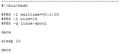
The command qsub [file name], executed on the master, starts a job. To run a job, you need a Bash file. In the example above, the date is displayed, wait 10 seconds and then again output the date. The result is then stored in the directory on the master from which the job was started.
Useful Commands
There are some commands in Torque with which you can trace the running jobs and which are very useful for troubleshooting.
The command
pbsnodes -a
, executed on the master, shows if a node is active or not. With the command
qstat
a list of running or finished jobs is displayed.

There you can see which number a job has which node is used and whether the job is started, in progress or has already ended.
A very useful command for debugging is
tracejob [job number]
This is a command from Torque which searches and summarizes the log files in the pbs_server, mom and scheduler. With this one gets a quick overview
ARM-Cluster (German)
Wir erklären, wie wir ein einfachen Cluster aus 5 Banana Pis gebaut haben und ob sich günstige ARM-Rechner als Clustereinheiten lohnen. (Jonas Gresens, Lennart Bergmann, Rafael Epplee)
Projektziel
Das ursprüngliche Ziel war der Bau einen lauffähigen Cluster aus Einplatinencomputern (wie z.B. Raspberry Pis). Das ganze Projekt dient daher als Machbarkeits- bzw. Brauch- barkeitsstudie von einem kostengünstigen Cluster auf Basis der ARM-Architektur, insbesondere im Hinblick auf Stromeffizienz und Softwareunterstützung. Ein Anwendungsszenario für einen solchen Cluster wäre beispielsweise die Ausführung von Tests im kleineren Maßstab auf echter Hardware. Es war geplant, CoreOS als Betriebssystem und Docker zur Organisation der Anwendungen zu verwenden, da diese Kombination einen einfachen beständigen Betrieb des Clusters versprechen zu schien. Zum Schluss sollte der Cluster, samt aller zugehöriger Hardware, in einem, für Serverschränke genormten, Plexiglas-Gehäuse Platz finden, damit er in das Cluster-Rack der Arbeitsgruppe eingebaut werden kann.
Hardware
Board
Als Erstes mussten wir uns Gedanken über die Wahl des Einplatinen-ARM-Computers machen. Dazu haben wir die verschiedenen Boards mit einander verglichen:
| Board | Raspberry Pi 2 | BeagleBone Black | Cubieboard4 | Banana Pi M2 |
| CPU | Cortex A7 | Cortex A8 | Cortex A7/A15 | Cortex A7 |
| Architektur | ARMv7 | ARMv7a | ARMv7/ARMv7 | ARMv7 |
| Kerne | 4 | 1 | 4/4 | 4 |
| Taktrate | 900 MHz | 1000 MHz | 1300/2000 MHz | 1000 MHz |
| RAM | 1 GiB DDR2 | 512 MiB DDR3 | 2 GiB DDR3 | 1 GiB DDR3 |
| Netzwerk | bis 100 Mbit/s | bis 100 Mbit/s | bis 1000 Mbit/s | bis 1000 Mbit/s |
| Kosten | 40 Euro | 55 Euro | 100 Euro | 60 Euro |
Mit vier Kernen á 2 GHz, 2 GiB DDR3 RAM und Gigabit-Ethernet ist das Cubieboard4 unschwer als das Leistungsstärkste der vier aufgeführten zu erkennen. Der Preis von 100 ist für die Leistung zwar komplett angemessen, für unser Projekt jedoch etwas zu hoch, sodass das Cubieboard4 leider aus der engeren Auswahl fiel. Anders beim BeagleBone Black, hier passt der Preis von nur 55,00Euro, leider kann das Board leistungstechnisch nicht mit den beiden anderen verbliebenden Boards mithalten. Mit nur einem Kern und 512 MB RAM, steht es klar hinten an. Der Raspberry Pi 2 (Modell B) besitzt zwar einen Preisvorteil gegenüber dem Banana Pi M2, hat dafür aber auch nur DDR2 statt DDR3 RAM und eine 100 MHz niedrigere Taktfrequenz. Ausschlaggebend war am Ende die höhere Netzwerkdurchsatzrate des Banana Pi M2, der mit 1000Mbit/s aufwarten kann. Wir haben uns für fünf Banana Pis entschieden, vier Compute-Nodes und ein Head-Node.
Weitere Komponenten
- SD-Karten - Da die meisten nötigen Komponenten des Clusters nur auf dem Head installiert werden sollten, haben wir für diesen eine 32GB Micro-SD-Karte besorgt und für die Nodes, auf denen eigentlich nur die Berechnungen stattfinden sollen und nicht viel installiert sein muss, vier 8 GB Karten.
- Switch - Wir haben uns für einen D-Link DGS-10008D Switch entschieden, ausschlaggebend waren hierbei das Gigabit LAN sowie die 8 Ports, so dass alle Compute-Nodes + Head-Node gleichzeitig am Switch, und dieser auch noch am Internet angeschlossen werden kann.
- Stromversorgung - Ein Banana Pi soll bei Höchstleistung nicht mehr als 5 Watt benötigen, deshalb haben wir uns bei der Stromversorgung für einen USB-Port von Logilink entschieden, der 50 Watt Leistung bringt und sechs USB-Anschlüsse hat. Damit hatten wir über die Dauer des Projekts auch keine Schwierigkeiten, was den Energieverbrauch angeht.
- Case - Unser Cluster hat noch kein Case in dem die ganze Hardware unterkommt, allerdings gibt es ein 3D-gedrucktes Case in dem sich die Banana Pis befinden, sodass diese nicht lose herumliegen. Das Case ist ursprünglich für Raspberry Pis gedacht, die Maße des Banana Pis sollen laut Hersteller aber gleich dem der Raspberrys sein. Wie wir leider herausfinden mussten entspricht dies nicht ganz der Wahrheit, die Banana Pis sind etwas größer. Das Case musste daher von Hand angepasst werden. Die Banana Pis passen nun hinein, sitzen aber nicht so gut und fest wie es Raspberry Pis tun würden.

System-Aufbau
OS
Eines unserer primären Ziele war es, die Anbindung neuer Compute Nodes so einfach wie möglich zu machen. Zusätzlich sollte der Cluster für eine breite Menge an Anwendungen zur Verfügung stellen. Für solche Anforderungen bietet sich CoreOS besonders an:
- Verteiltes,automatisches Konfigurationsmanagement über etcd (inklusiveIP-Adressen- Vergabe)
- Isolierte Umgebungen mit individuellen Abhängigkeiten für jede Anwendung über Container (rkt)
- Anwendungsverwaltung á la Slurm über fleet
Leider wird die ARM-Architektur, wie wir schnell herausfanden, (noch) nicht von CoreOS unterstützt. Somit entschieden wir uns gegen CoreOS und beschlossen, die Lösung für unsere Anforderungen auf einer anderen Ebene als dem Betriebssystem zu suchen. Auf den Banana Pis läuft nun die Raspbian-Distribution, zu finden auf der offiziellen Banana-Pi-Homepage.[19]
Verkabelung
Der Aufbau des Clusters ist verhältnismäßig simpel. Die 5 Banana Pis werden, sowohl Head als auch Compute Nodes, direkt mit dem Switch verbunden. Vom Switch geht ein Netzwerkkabel in das umliegende Netzwerk. Der USB-Port liefert über 6 Ausgänge Strom, durch 5 davon werden die Banana Pis versorgt, an den 6. wird der Switch angeschlossen.
Netzwerk
Die Topologie unseres Clusters ist, wie im vorigen Abschnitt bereits zu erahnen, etwas ungewöhnlich. Bei den üblichen Clustern ist die Head Node über ein Interface an das umliegende Netzwerk und über ein anderes an den Switch und damit die restlichen Compute Nodes angebunden. Das bedeutet, dass jede Kommunikation von den Compute Nodes nach außen über die Head Node geht. Oft wird diese Topologie genutzt, um ein lokales Netzwerk zwischen den Compute Nodes aufzubauen und Kommunikation der Compute Nodes nach außen zu unterbinden. Die Head Node vergibt in diesem Fall über DHCP lokale IP-Adressen an die Compute Nodes. Diese Herangehensweise vereinfacht sowohl das Management der Compute Nodes als auch die Zugriffskontrolle auf den Cluster. Da ein Banana Pi allerdings nur einen Netzwerk-Anschluss hat, verwendet unser Cluster eine leicht abgewandelte Version dieser Topologie, wie die Abbildung zeigt. Über den Switch sind alle Nodes mit dem umliegenden Netzwerk verbunden. Statt zwei echten Netzwerk-Interfaces hat die Head Node ein virtuelles Interface, das die Verbindung zum lokalen Netzwerk darstellt. Dieses Setup funktioniert zwar, verlässt sich allerdings darauf, dass die Compute Nodes sich nicht zufällig über die direkte Verbindung an das umliegende Netz von einem anderen DHCP-Server eine IP-Adresse besorgen. Um dem Vorzubeugen, sind die Compute Nodes in unserem Fall auf der Blacklist des äußeren DHCP-Servers eingetragen und werden von ihm ignoriert. Als DHCP-Server auf der Head Node verwenden wir dnsmasq, in dessen Konfigurationsdateien die einzelnen Compute Nodes über die Option dhcp-host per MAC-Adresse mit einer festen IP assoziiert werden.
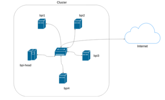
NFS
Da wir fast alle Daten mölichst zentralisiert auf der Head-Node speichern, verwenden wir NFS um diese den Compute-Nodes über das Netzwerk als POSIX-kompatibles Dateisystem zugänglich zu machen:
- Auf der Head-Node läuft der NFS-Server, der /srv und /home bereitstellt.
- Auf jeder Compute-Node läuft ein NFS-Client, sodass die home-Verzeichnisse auf dem Head per fstab auf den Compute-Nodes gemountet werden können und die Compute-Nodes ihre lokalen Packages mit dem Golden Image auf dem Head synchronisieren können.
# /etc/exports: the access control list for filesystems which may be exported # to NFS clients. See exports(5).
/srv *(rw,sync,no_subtree_check,no_root_squash)
/home *(rw,sync,no_subtree_check)
proc            /proc
/dev/mmcblk0p1  /boot
/dev/mmcblk0p2  /
proc    defaults          0       0
vfat    defaults          0       2
ext4    defaults,noatime  0       1
bpi-head:/home
-> async,rw,relatime,rsize=1048576,
wsize=1048576,proto=tcp,intr,nfsvers=3
Golden Image
Cluster setzen sich aus mehreren einzelnen Rechnern zusammen und sind daher in ihrer Administration deutlich aufwändiger als ein einzelnes System. Um diese dennoch möglichst einfach zu halten, wird für alle Compute-Nodes nach Möglichkeit die gleiche Hardware verwendet und sämtliche Software der Compute-Nodes (inklusive Betriebssystem) zentral gespeichert und übers Netzwerk bereitgestellt. Das auf der Head-Node gespeicherte Systemabbild wird als “Golden Image” bezeichnet und stellt den gemeinsamen aktuellen Zustand aller Compute-Nodes dar. Durch das Golden Image müssen effektiv nur noch zwei verschiedene Systeme administriert werden, was die Skalierbarkeit des Cluster-Setups drastisch steigert indem es den Aufwand für die Verteilung von neuer Software und deren Konfiguration konstant hält. Die Compute-Nodes der meisten handelsüblichen Cluster booten per PXE direkt das, im Netzwerk bereitgestellte, Golden Image. Banana Pis können jedoch nicht per PXE über das Netzwerk gebootet werden, weil ihr BIOS so konfiguriert ist, dass es den Bootloader auf der SD-Karte benutzt, weswegen wir einen kleinen Umweg gehen mussten:
- Die SD-Karte einer jeden Compute-Node enthält ein komplett lauffähiges System, das beim Einschalten gebootet wird.
- Alle Daten auf der SD-Karte stammen aus dem Golden Image. Die Installationen unterscheiden sich nur in ihrem hostname.
- Wir verteilen Änderungen am Golden Image nicht direkt beim Reboot, sondern indem wir semiautomatisch per Skript die lokale Installation mit dem Golden Image synchronisieren.
- Die SD-Karten neuer Compute-Nodes können ebenfalls per Skript mit dem aktuellen Zustand des Golden Image geflasht werden, sodass der Cluster einfach erweiterbar bleibt.
Skripte
Im folgenden werden unsere drei selbstentwickelten Skripte zur Verwaltung und Nutzung des Golden Image vorgestellt:
create-local-installation.sh
- Komplett neue Installation des aktuellen Golden Image für eine neue/kaputte Node
- Ausführung auf einem extra Gerät (z.B. Laptop) mit SD-Karten-Slot
- Funktionsweise: erzeugt neue Partitionstabelle, erzeugt Dateisysteme, kopiert Bootloader, kopiert Inhalt des Golden Image mit rsync über NFS von der Head-Node
update-local-installation.sh
- Aktualisierung der lokalen Installation auf einer bereits installierten Node
- Ausführung auf der laufenden Compute-Node
- Funktionsweise: kopiert alle geänderten neuen Dateien mit rsync über NFS aus dem Golden Image
start-chroot.sh
- Wrapper-Skript für die Administration des Golden Image per chroot-Environment
- Ausführung auf der Head-Node, nur eine Instanz gleichzeitig möglich
- Funktionsweise: mounten aller benötigten Partitionen, starten einer bash im chroot für den Nutzer
Container
Trotz unserer Entscheidung gegen CoreOS gefiel uns die Idee der Anwendungsisolierung über Container. Im Gegensatz zu virtuellen Maschinen bringen Container weniger Performanceeinbußen mit sich, was uns bei der ohnehin schon unterdurchschnittlichen Leistung der Banana Pis besonders gelegen kam.
Docker
Da Docker momentan die beliebteste Container-Implementation darstellt, begannen wir hier mit unseren Installationsversuchen. Docker verwendet einige neue Features des Linux-Kernels, die in der offiziellen Raspbian- Distribution für den Banana Pi nicht enthalten sind. Die exzellente Arch-Linux-Distribution für ARM2 unterstützt diese out of the box, da der restliche Cluster des DKRZ allerdings komplett auf Debian-basierten Systemen läuft, wurde beschlossen, für einfachere Maintenance auch auf unserem Cluster ein solches System zu verwenden. Auch auf Raspbian soll es möglich sein, Docker zum laufen zu bringen, allerdings braucht man dort einen selbst kompilierten, neueren Kernel. Im Prinzip kein Problem - leider brauchen die Banana Pis einen speziellen, eigenen Kernel vom Hersteller LeMaker3. Der Quelltext wurde erst vor kurzem von LeMaker bereitgestellt[20] und ist noch bei Version 3.4, während Docker mindestens Version 3.10 braucht. Nach einer Menge Recherche und einem fehlgeschlagenen Versuch, einen aktuellen Linux-Kernel auf einem Banana Pi zu kompilieren, gaben wir also neben CoreOS auch Docker auf.
rkt
rkt ist eine alternative Container-Implementierung, entwickelt vom CoreOS-Team. rkt hat zwar keine offizielle Unterstützung für die ARM-Architektur - das hinderte uns allerdings nicht daran, das Projekt selber zu kompilieren. Dabei kam dann heraus, dass rkt leider auch (noch) keine 32-bit-Systeme unterstützt, was das Projekt auf den ARMv7-Prozessoren der Banana Pis nicht lauffähig macht.
systemd-nspawn
Nach unseren Versuchen mit Docker und rkt legten wir unsere letzte Hoffnung auf das systemd-initsystem. Das hat seit einiger Zeit eine minimale Container-Implementierung, genannt systemd-nspawn.[21] Ursprünglich für schnelle Tests von systemd selber gedacht, enthält es inzwischen die grundlegendsten Features und hätte für unsere Zwecke vollkommen gereicht. Gegen Ende unseres Projekts fingen wir damit an, systemd testweise auf einem Banana Pi zu installieren (unsere Version von Raspbian verwendete noch klassische initscripts). Die Installation endete jedoch jedes mal mit einem nicht bootenden Banana Pi, einer unbrauchbaren Raspbian-Installation und einem zeitaufwändigen neuflashen der SD-Karte. An diesem Punkt des Projekts hatten wir leider nicht mehr genug Zeit, um diesen Fehler zu beheben.
Installierte Software
Nachdem unseren Cluster endlich lauffähig war, wollten wir die tatsächliche Leistungsfähigkeit der Banana Pis mit der HPL-Benchmark[22] testen. HPL benötigt eine MPI- und eine BLAS-Bibliothek, die wir daher ebenfalls installieren mussten.
MPI
Der “Message Passing Interface”-Standard (MPI) beschreibt den Nachrichtenaustausch zwischen einzelnen parallel Prozessen, die gemeinsam an der Lösung eines Problems arbeiten. MPI legt dabei kein konkretes Protokoll oder Implementierung fest, sondern beschreibt die Semantik der verschiedenen Arten von Kommunikations-Operationen und ihre API, sodass die eigentliche Nutzung des Standards eine MPI-Implementierung benötigt. Anfänglich wollten wir OpenMPI oder MVAPICH2 nutzen, die jedoch aus verschiedenen Gründen beide nicht funktionierten:
- OpenMPI ließ sich nicht vollständig kompilieren, da es auf ARM nicht lauffähigen Assembler-Code enthielt und der Portierungsaufwand sich vermutlich nicht gelohnt hätte.
- MVAPICH2 funktionierte bis zu einem bestimmten Systemupdate einwandfrei, danach ließ sich jedoch der ”libpmi“-Header nicht mehr finden.
Aus der Not heraus entschieden wir uns daher dazu ein schon vorkompiliertes MPICH2 aus den Paketquellen unserer Distribution zu benutzen, da wir an dieser Stelle davon ausgingen, dass sich die Wahl der MPI-Implementierung für unseren Cluster wenn überhaupt nur sehr gering in der gemessenen Leistung widerspiegeln würde.
OpenBLAS
Die “Basic Linear Algebra Subprograms” (BLAS) sind eine Sammlung von Routinen für grundlegende Vektor- und Matrix-Operationen. Das von uns genutzte OpenBLAs[23] ist eine optimierte BLAS-Bibliothek und musste zur Nutzung auf den Banana Pis neu kompiliert werden. Das Kompilieren von OpenBLAS auf dem Pi hat ca. 1 Stunde gedauert. Die besten Messergebnisse haben wir mit einer Version ohne Threading (mittels USE THREADING=0) erzielt.
HPL
Die “High-Performance Linpack”-Benchmark ist ein Programm zur Messung der Fließkomma-Rechenleistung eines (verteilten) Computer-Systems. HPL misst die Leistung des Systems in GFLOPS indem es ein dichtes -System von linearen Gleichungen löst und errechnet die Leistung in GFLOPS. Wie OpenBLAS mussten wir HPL speziell für unser System kompilieren, damit es möglichst effizient an die verfügbare Hardware angepasst ist.


Messergebnisse
HPL hat vier verschiedene Hauptparameter:
- gibt die Höhe und Breite der Matrix an, das Problem wächst quadratisch mit
- ist die Nachrichtengröße bei der Kommunikation zwischen den Prozessen
- und beschreiben die Aufteilung der Matrix auf das Prozessgitter


Die vier Kurven zeigen das Verhältnis der gemessenen Performance mit verschiedenen vielen Compute-Nodes und Problemgrößen: Der schwache Speedup (bei gleich großem Problem pro Kern) ist in Anbetracht der verwendeten Hardware überraschend gut (ungefähr 2.8 bei 3 verwendeten Compute-Nodes) Die Entwicklung des starken Speedups (bei fester Problemgröße trotz steigender Anzahl der Kerne) zeigt jedoch, dass sich der verwendete handelsübliche Switch nicht für HPC eignet, da mit steigender Zahl an Compute-Nodes die Leistung einbricht. Leider konnten wir keine Leistungsdaten für weitere HPL-Runs mit größerem auf 4 Nodes messen, da es technische Probleme gab:
- bpi4 schaltete sich bereits nach wenigen Minuten unter Volllast ab.
- bpi-head konnte nicht als Ersatz verwendet werden, da er die gleichen Symptome zeigte.
Die Instabilität der Pis bei großer Hitze stellt ein großes Problem für einen tatsächlich intensiv genutzten Pi-Cluster dar.
SLURM
SLURM[24] steht für Simple Linux Utility for Resource Management und ist ein Open Source Workload Manager, der auf vielen Clustern und Supercomputern rund um die Welt verwendet wird. SLURM wird dazu verwendet, einzelne Jobs möglichst effizient auf die Knoten des Clusters zu verteilen. Obwohl wir uns sehr bemüht haben, gab es im Laufe des Projekt wesentlich mehr Komplikationen als wir erwartet haben und so fehlte uns am Ende die Zeit dafür, SLURM komplett in den Cluster zu integrieren.
Status Quo
Aktueller Stand
Zum jetzigen Zeitpunkt haben wir einen zwar nicht optimalen aber funktionierenden Cluster. Wir benutzen ein Golden Image, mit dessen Hilfe es ein leichtes ist, alle Knoten auf den selben Stand zu bringen, und durch welches der Cluster einfach um zusätzliche Knoten erweiterbar ist. Die Netzwerkeinbindung ist noch suboptimal, da Compute-Nodes in manchen fällen eine IP aus dem Internet, statt von der Head-Node beziehen, wo durch sie von dieser nicht ansprechbar sind. Auf der positiven Seite, kann der Cluster mit nutzbaren MPI-Libraries, sowie lauffähigem HPL aufwarten, womit ausführliche Leistungstests möglich sind. Die Banana Pis befinden sich in einem eigens dafür 3D-gedrucktem Case, welches leider ein bisschen klein geraten ist.
Weiterführende Arbeit
Die Lösung Netzwerk-Problematik wären statische IPs, sodass keine Knoten mehr eigenwillig auf IP-Suche gehen können. Für eine möglichst vollständige Integration in den WR-Cluster müssten nur noch ein paar wenige Softwarepakete hinzugefügt werden:
- miit SLURM bleibt das (vom WR-Cluster) gewohnte UI zur Nutzung des Clusters erhalten.
- auf dem WR-Cluster wird LDAP zum Zugriff auf die Home-Verzeichnisse der Nutzer verwendet und wird daher zwingend auf dem Pi-Cluster benötigt um die Problematik mehrerer Home-Verzeichnisse pro Nutzer zu umgehen.
- das Monitoring-Tool Ganglia ist zwar im allgemeinen optional, sollte aber auch vorhanden sein, da es wie SLURM ebenfalls zur gewohnten UI gehört.
Außerdem fehlt für den Einbau in diesen Cluster ein Plexiglas-Gehäuse in dem die ARM-Computer sowie das gesamte Zubehör, einige LEDs und Lüfter Platz finden.
Fazit
Der Banana Pi
Nach einiger Erfahrung mit dem Modell “Banana Pi” möchten wir hier einen kurzen Überblick über Vor- und Nachteile des Modells geben. Da wir aus der Perspektive des HPC an dieses Projekt gegangen sind, waren für uns die Hardware-Aspekte bei der Planung besonders wichtig. Im Besonderen versprach der Banana Pi durch das Gigabit-Ethernet eine problemfreie Kommunikation zwischen den Compute Nodes, auch mit den für HPC üblichen großen Datenmengen. Tatsächlich konnten wir in unseren Benchmarks auch keine Probleme mit der Kommunikationslast erkennen. Zusätzlich ergaben unsere Vergleiche mit einem Raspberry Pi 2 Modell B gerade mal einen Performanceunterschied von etwa 300 MFLOPS. Schnell mussten wir jedoch feststellen, dass die eher kleine Community undd as Ökosystem um den Banana Pi einige Probleme mit sich bringen. Zum einen mussten wir feststellen, dass es tatsächlich verschiedene Hersteller gibt, die alle von sich behaupten, den “offiziellen” Banana Pi zu fabrizieren. Mit jedem dieser Hersteller kam eine leicht andere Dokumentation mit vielen fehlenden Stellen. SD-Karten-Images für den Raspberry Pi funktionieren mit dem Banana Pi nicht; Es bleibt unklar, ob es eine tatsächlich offizielle Seite mit offiziellen Linux-Distributionen gibt. Lange Zeit war der modifizierte Linux-Kernel für den Banana Pi nicht quelloffen; Nach viel Druck aus der Community wurde der Code dann doch veröffentlicht.[25] Leider ist das letzte stabile Release dieses Kernels noch bei Version 3.4. Das machte unter Anderem das kompilieren eines eigenen Kernels für die Docker-Installation unmöglich.
Andere Vor- und Nachteile
Eine der Fragen, die wir mit unserem Projekt beantworten wollten, war die Frage nach der Stromeffizienz der Banana Pis, insbesondere im Kontext des High Performance Computing. Leider enttäuscht der ARM-Cluster in dieser Hinsicht. Wenn wir eher konservativ [26] von einem Verbrauch von 5 Watt (unter voller Last) ausgehen, entspräche das bei unseren Benchmarks ungefähr GFLOPS pro Watt. Laut der TOP500-Liste sind Werte im Bereich von 2 GFLOPS pro Watt der aktuelle Stand der Technik.[27] Trotz des geringen Preis eignet sich ein Cluster aus Banana Pis nichtmal gut für das Testen von Programmen in kleinem Maßstab, da die ARM-CPU nicht alle Befehlssätze einer x86(64)-CPU unterstützt und daher für Probleme bei der Kompilierung sorgt - die Nutzung eines virtualisierten Clusters (z.B. via Vagrant) ist deutlich komfortabler. Im Allgemeinen kann man also sagen, dass sich ein ARM-Cluster unserer Erfahrung nach hauptsächlich lohnt, um in einem möglichst realistischen Szenario Aufbau und Installation eines Clusters zu üben. Die Skripte zur Verwaltung der verschiedenen Nodes funktionieren exzellent und können ohne Probleme in jedem Projekt, das mit mehreren Pi-artigen Computern arbeitet, zur einfachen Administration verwendet werden.

Appendix
create-local-installation.sh
#!/bin/bash
# JG/RE/LB 2015

if [[ $# -ne 4 ]]; then
        echo "Usage: $0 bpi_head_ip dist device hostname"
        exit 1
fi

if [ "$USER" != "root" ]; then
        echo "MUST be run as root! Try 'sudo $0 ...'"
    exit 1
fi

BPI_HEAD_IP="$1"
DIST="$2"
DEV="$3"
HOSTNAME="$4"

# sd card formatting
echo "Partitioning $DEV"
parted -s $DEV mklabel msdos || exit 1
parted -s $DEV unit s mkpart primary fat32 8192s 122879s || exit 1
parted -s -- $DEV unit s mkpart primary 122880s -1s || exit 1
echo "Report:"
fdisk -l $DEV

echo "Filesystems:"
mkfs.vfat -F 32 ${DEV}p1 || exit 1
mkfs.ext4 ${DEV}p2 || exit 1

echo "Bootloader"
dd if="$(dirname $0)"/bootloader_ohne_table.img count=2048 of=/dev/mmcblk0 seek=8 bs=1024

# mounting
mkdir /tmp/target/{b,r}oot -p
mount ${DEV}p1 /tmp/target/boot
mount ${DEV}p2 /tmp/target/root

# rsync magic
rsync -axzh --stats root@$BPI_HEAD_IP:/srv/nodes/$DIST/boot/ /tmp/target/boot || exit 1
rsync -axzh --stats root@$BPI_HEAD_IP:/srv/nodes/$DIST/root/ /tmp/target/root || exit 1

echo $HOSTNAME > /tmp/target/root/etc/hostname

# Clean up
umount /tmp/target/*
update-local-installation.sh
#!/bin/bash
# JG/RE/LB 2015

test -z "$1" && echo "Please specify a distribution." && exit 1

DIST="$1"

#####
# mounting the source, this could be done outside of this script to use arbitrary sources.
mkdir -p /tmp/source_root
umount /tmp/source_root
mount -o ro,nfsvers=3 bpi-head:/srv/nodes/$DIST/root /tmp/source_root || exit 1

mkdir -p /tmp/source_boot
umount /tmp/source_boot
mount -o ro,nfsvers=3 bpi-head:/srv/nodes/$DIST/boot /tmp/source_boot || exit 1

####
# Sanity checks to check if the ip is 10.0.0.X where X below 100, then the script is allowed to run.

IP=$(ip addr show dev eth0 |grep "inet " |sed "s/.* inet \([0-9.]*\)\/.*/\1/")

if [[ ${#IP} -lt 8 ]] ; then
        echo "Could not determine IP!"
        exit 1
fi

LAST=${IP#10.0.0.}
if [[ $IP == $LAST || $LAST -gt 99 ]] ; then
        echo "Invalid host with IP: $IP"
        echo "I won't run the script on this machine!"
        exit 1
fi

rsync -axzh --delete --exclude="/home" --ignore-errors --progress /tmp/source_root/ /
rsync -axzh --delete --exclude="/home" --ignore-errors --progress /tmp/source_boot/boot

hostname > /etc/hostname

# cleanup and restoring the previous state
umount /tmp/source_root
umount /tmp/source_boot
start-chroot.sh
#!/bin/bash
# JG/RE/LB 2015

(
flock -n 200
CHROOTDIR="/srv/nodes/default/root"

usage ()
{
    echo "USAGE: ${0} [-h|--help] [<DIR>]"
    echo
    echo "-h"
    echo "  --help     print this message"
    echo "<DIR>  directory with common file system"
    echo
}

if [[ "$1" != "" ]] ; then
        CHROOTDIR="/srv/nodes/${1}/root"
fi
[ -d "${CHROOTDIR}" ] || \
        { echo "Directory for chroot ${CHROOTDIR} not found!" && exit 1; }

echo "Starting chroot environment in ${CHROOTDIR}"

# mount dev
[ -d ${CHROOTDIR}/dev ] &&
mount -o bind /dev ${CHROOTDIR}/dev

# mount dev/pts
[ -d ${CHROOTDIR}/dev/pts ] &&
mount -o bind /dev/pts ${CHROOTDIR}/dev/pts

# mount /run for resolv.conf
[ -d ${CHROOTDIR}/run ] &&
mount -o bind /run ${CHROOTDIR}/run

# mount boot 'partition'
mount -o bind ${CHROOTDIR}/../boot ${CHROOTDIR}/boot

# mount proc
[ -d ${CHROOTDIR}/proc ] &&
mount -t proc proc_chroot ${CHROOTDIR}/proc

# mount sysfs
[ -d ${CHROOTDIR}/sys ] &&
mount -t sysfs sysfs_chroot ${CHROOTDIR}/sys

#JK:
#sed -i "s/10.0.0.250/129.206.100.126/" ${CHROOTDIR}/etc/resolv.conf if [ -f ${CHROOTDIR}/usr/sbin/invoke-rc.d ]
then
        echo '#!/bin/sh' > ${CHROOTDIR}/usr/sbin/policy-rc.d
        echo 'exit 101' >> ${CHROOTDIR}/usr/sbin/policy-rc.d
        chmod +x ${CHROOTDIR}/usr/sbin/policy-rc.d
fi

/usr/sbin/chroot ${CHROOTDIR} /bin/bash

# YOU ARE IN CHROOT HERE AND THIS SCRIPT IS STOPPED UNTIL YOU QUIT BASH!

echo "Closing chroot environment!"

[ -f ${CHROOTDIR}/usr/sbin/policy-rc.d ] &&
rm ${CHROOTDIR}/usr/sbin/policy-rc.d

# umount sysfs
mountpoint -q ${CHROOTDIR}/sys && umount sysfs_chroot

# umount proc
mountpoint -q ${CHROOTDIR}/proc && umount proc_chroot

# umount boot 'partition'
# 'mountpoint' doesn't work here for some reason umount ${CHROOTDIR}/boot

# umount dev/pts
mountpoint -q ${CHROOTDIR}/dev/pts && umount ${CHROOTDIR}/dev/pts

# umount /run
mountpoint -q ${CHROOTDIR}/run && umount ${CHROOTDIR}/run

# umount dev/pts
mountpoint -q ${CHROOTDIR}/dev && umount ${CHROOTDIR}/dev
) 200>/var/lock/start-chroot.sh
SLURM Konfiguration
ControlMachine=bpi-head ControlAddr=10.0.0.250
#
MailProg=/usr/bin/mail
MpiDefault=none
#MpiParams=ports=#-#
ProctrackType=proctrack/cgroup
ReturnToService=1
SlurmctldPidFile=/var/run/slurmctld.pid
#SlurmctldPort=6817
SlurmdPidFile=/var/run/slurmd.pid
#SlurmdPort=6818
SlurmdSpoolDir=/var/spool/slurmd
SlurmUser=slurm
#SlurmdUser=root
StateSaveLocation=/var/spool/slurm
SwitchType=switch/none
TaskPlugin=task/none
#
# TIMERS
#KillWait=30
#MinJobAge=300
#SlurmctldTimeout=120
#SlurmdTimeout=300
#
# SCHEDULING
FastSchedule=1
SchedulerType=sched/backfill
#SchedulerPort=7321
SelectType=select/linear
#
# LOGGING AND ACCOUNTING
AccountingStorageType=accounting_storage/none
ClusterName=pi-cluster
#JobAcctGatherFrequency=30
JobAcctGatherType=jobacct_gather/none
#SlurmctldDebug=3
SlurmctldLogFile=/etc/slurm-llnl/slurmctldLog.log
#SlurmdDebug=3
SlurmdLogFile=/etc/slurm-llnl/slurmdLog.log
#
# COMPUTE NODES
NodeName=bpi[1-4] CPUs=4 State=UNKNOWN
PartitionName=debug Nodes=bpi[1-4] Default=YES MaxTime=INFINITE State=UP
Bibliography
[BC08] Rory Bray and Daniel Cid. OSSEC Host-Based Intrusion Detection Guide. Syngress Media, 2008.
List of Figures
1.1 Schematic HPC Cluster
4.1 Overview of the cluster and software
4.2 The plugins (services) used to monitor a local host by default
4.3 Node configuration consists of two parts: host and services specification.
4.4 Overview of used ICINGA components
4.5 Overview over monitored services by our test setup
4.6 Overview of used Ganglia components
4.7 Front page of Ganglia
4.8 Enter a host regular expression to only visualize data of interesting nodes
4.9 A custom aggregated graph with with the nodes specified in figure 4.8
4.10 Dialogue to create custom aggregated graphs
4.11 A custom aggregated graph created by the dialogue presented in figure 4.10.
5.1 Infrastructure SLURM with the two most important services
5.2 Auswirkungen von FIFO und Backfill Strategien
7.1 Infrastructure of OSSEC. This is only an extract of the whole infrastructure.
7.2 The analysis process of an event in OSSEC [BC08]
7.3 The WUI’s main window
7.4 Searching for alerts in a period from 16 February 2013 to 25th march
2013. Only alerts with a minimum severity level of seven are shown.
7.5 Latest modified files for all agents and servers sorted by date.
7.6 Modified files for a particular agent (worker1). The configuration files
ossec.conf and internal_options.conf have changed
7.7 Statistics for the 25th March 2013. It shows which and how many rules
were found for specific events and how much rules were found with a
certain severity level.
7.8 Representation of an event with in the OSSEC WUI.
9.1 Setting MySQL root password
9.2 setting IP address for the network to protect
9.3 Database setup for Snort
9.4 BASE configuration
9.5 Setting Passwort for the database administrator
9.6 setting front-end access
10.1 Interaction between managers and sensors
10.2 Possible third party sensors
10.3 IMPORTANT [NODE-ADDRESS] must be commented
10.4 The manager now waits for the password
10.5 The by the sensor generated password must now be entered in the manager
10.6 Registration successful!
10.7 In the web interface we see the sensors used and the manager
10.8 In the web interface we see all the messages the the auth.log file provides.
12.1 Configure Bug Fix
12.2 Configure Bug Fix 2
12.3 Config file
12.4 Tracejob error
12.5 Bash file example
12.6 qstat display
13.1 Das Herz unseres Clusters: 5 Banana Pis in einem 3D-gedruckten Case
13.2 Netzwerktopologie des Clusters
13.3 Messergebnisse mit HPL
List of Tables
5.1 Default values for QOS
7.1 Example of a predecoded ssh event
13.1 My caption
Listingverzeichnis
2.1 Install python-software-properties for the command add-apt-repository
2.2 Add the ppa repository
2.3 Update the package database
2.4 Install the desired packages
4.1 Suggested order of packages to install Icinga on Ubuntu
4.2 NRPE check command in worker configuration file
4.3 Add the IP address of the master to /etc/nagios/nrpe.cfg
4.4 Add custom commands to /etc/nagios/nrpe_local.cfg
4.5 Check if NRPE is setup correctly with check_nrpe
4.6 check_nrpe: success!
4.7 Integrating RRDTool into the environment
4.8 Installation of Ganglia
4.9 Interesting parts of gmetad.conf
4.10 Configuration of gmond_master.conf
4.11 Configuration of gmond_collector.conf
4.12 Configuration of gmond_worker.conf
5.1 Ausgabe des sinfo Befehls
5.2 srun interaktiv
5.3 srun Command with some options
5.4 scancel Command with some options
5.5 Ausgabe des squeue Befehls
5.6 Using the scontrol command
5.7 Example for a jobscript
6.1 Configuration for master
6.2 Configuration of the hosts for master
6.3 Configuration for workers
6.4 Configuration of the hosts for worker
7.1 Example of a decoder for ssh
7.2 Getting the OSSEC source code
7.3 Extracting the archive and starting the installation
7.4 Starting OSSEC
7.5 Installing the mail server and an email program
7.6 Configuring the email notification in OSSEC
7.7 Setting the email alert level
7.8 Starting the key management
7.9 Adding an agent
7.10 Setup of OSSEC on the agent’s side. The only difference is the setting of
the server’s IP address
7.11 Generating the key for an agent (worker1)
7.12 Importing the key of the agent (worker1) generated on the server
7.13 Success of the setup of the agent
7.14 Installing the apache server and php5
7.15 Getting the WUI sources
7.16 Extracting the wui files, moving it to /var/www and starting the setup
7.17 Installing the WUI
7.18 Adding user www-data to ossec group
10.1 Database name and user (example)
10.2 Apache configuration for Prewikka
References
- ↑ http://www.gnu.org/software/automake/
- ↑ http://www.cmake.org/
- ↑ https://code.google.com/p/waf/
- ↑ Long Term Support
- ↑ https://www.icinga.org/
- ↑ https://launchpad.net/ formorer/+archive/icinga
- ↑ Secure Shell
- ↑ Nagios Remote Plugin Executor
- ↑ http://docs.icinga.org/latest/en/pluginapi.html
- ↑ http://ganglia.sourceforge.net/
- ↑ http://oss.oetiker.ch/rrdtool/
- ↑ [foot:top500]http://www.top500.org/system/177999
- ↑ [foot:daemon] daemon - disk and execution monitor - On UNIX, a utility running in the background
- ↑ http://www.umbc.edu/hpcf/resources-tara/scheduling-policy.html
- ↑ http://www.adaptivecomputing.com/products/open-source/maui/
- ↑ http://www.ossec.net/doc/manual/rootcheck/manual-rootcheck.html
- ↑ http://www.ossec.net/
- ↑ http://www.postfix.org/
- ↑ http://bananapi.com/
- ↑ https://github.com/LeMaker/linux-sunxi
- ↑ http://www.freedesktop.org/software/systemd/man/systemd-nspawn.html
- ↑ http://www.netlib.org/benchmark/hpl/
- ↑ http://www.openblas.net/
- ↑ http://slurm.schedmd.com/
- ↑ https://github.com/LeMaker/linux-sunxi
- ↑ http://raspberrypi.stackexchange.com/questions/5033/how-much-energy-does-the-raspberry-pi-consume-in-a-day
- ↑ https://en.wikipedia.org/wiki/Performance_per_watt