Winding number
In mathematics, the winding number of a closed curve in the plane around a given point is an integer representing the total number of times that curve travels counterclockwise around the point. The winding number depends on the orientation of the curve, and is negative if the curve travels around the point clockwise.
- The term winding number may also refer to the rotation number of an iterated map.
Winding numbers are fundamental objects of study in algebraic topology, and they play an important role in vector calculus, complex analysis, geometric topology, differential geometry, and physics, including string theory.
Intuitive description

Suppose we are given a closed, oriented curve in the xy plane. We can imagine the curve as the path of motion of some object, with the orientation indicating the direction in which the object moves. Then the winding number of the curve is equal to the total number of counterclockwise turns that the object makes around the origin.
When counting the total number of turns, counterclockwise motion counts as positive, while clockwise motion counts as negative. For example, if the object first circles the origin four times counterclockwise, and then circles the origin once clockwise, then the total winding number of the curve is three.
Using this scheme, a curve that does not travel around the origin at all has winding number zero, while a curve that travels clockwise around the origin has negative winding number. Therefore, the winding number of a curve may be any integer. The following pictures show curves with winding numbers between −2 and 3:
 |
 |
 |
||
| −2 | −1 | 0 | ||
 |
 |
 |
||
| 1 | 2 | 3 |

Formal definition
A curve in the xy plane can be defined by parametric equations:

If we think of the parameter t as time, then these equations specify the motion of an object in the plane between t = 0 and t = 1. The path of this motion is a curve as long as the functions x(t) and y(t) are continuous. This curve is closed as long as the position of the object is the same at t = 0 and t = 1.
We can define the winding number of such a curve using the polar coordinate system. Assuming the curve does not pass through the origin, we can rewrite the parametric equations in polar form:

The functions r(t) and θ(t) are required to be continuous, with r > 0. Because the initial and final positions are the same, θ(0) and θ(1) must differ by an integer multiple of 2π. This integer is the winding number:

This defines the winding number of a curve around the origin in the xy plane. By translating the coordinate system, we can extend this definition to include winding numbers around any point p.
Alternative definitions
Winding number is often defined in different ways in various parts of mathematics. All of the definitions below are equivalent to the one given above:
Alexander numbering
A simple combinatorial rule for defining the winding number was proposed by August Ferdinand Möbius in 1865[1] and again independently by James Waddell Alexander II in 1928.[2] Any curve partitions the plane into several connected regions, one of which is unbounded. The winding numbers of the curve around two points in the same region are equal. The winding number around (any point in) the unbounded region is zero. Finally, the winding numbers for any two adjacent regions differ by exactly 1; the region with the larger winding number appears on the left side of the curve (with respect to motion down the curve).
Differential geometry
In differential geometry, parametric equations are usually assumed to be differentiable (or at least piecewise differentiable). In this case, the polar coordinate θ is related to the rectangular coordinates x and y by the equation:

Which is found by differentiating the following definition for θ:

By the fundamental theorem of calculus, the total change in θ is equal to the integral of dθ. We can therefore express the winding number of a differentiable curve as a line integral:

The one-form dθ (defined on the complement of the origin) is closed but not exact, and it generates the first de Rham cohomology group of the punctured plane. In particular, if ω is any closed differentiable one-form defined on the complement of the origin, then the integral of ω along closed loops gives a multiple of the winding number.
Complex analysis
Winding numbers play a very important role throughout complex analysis (c.f. the statement of the residue theorem). In the context of complex analysis, the winding number of a closed curve in the complex plane can be expressed in terms of the complex coordinate z = x + iy. Specifically, if we write z = reiθ, then


and therefore

As is a closed curve, the total change in ln(r) is zero, and thus the integral of is equal to multiplied by the total change in . Therefore, the winding number of closed path about the origin is given by the expression[3]


- .

More generally, if is a closed curve parameterized by , the winding number of about , also known as the index of with respect to , is defined for complex as[4]


- .

This is a special case of the famous Cauchy integral formula.
Some of the basic properties of the winding number in the complex plane are given by the following theorem:[5]
Theorem. Let be a closed path and let be the set complement of the image of , that is, . Then the index of with respect to ,


,

is (i) integer-valued, i.e., for all ; (ii) constant over each component (i.e., maximal connected subset) of ; and (iii) zero if is in the unbounded component of .


As an immediate corollary, this theorem gives the winding number of a circular path about a point . As expected, the winding number counts the number of (counterclockwise) loops makes around :
Corollary. If is the path defined by , then


Topology
In topology, the winding number is an alternate term for the degree of a continuous mapping. In physics, winding numbers are frequently called topological quantum numbers. In both cases, the same concept applies.
The above example of a curve winding around a point has a simple topological interpretation. The complement of a point in the plane is homotopy equivalent to the circle, such that maps from the circle to itself are really all that need to be considered. It can be shown that each such map can be continuously deformed to (is homotopic to) one of the standard maps , where multiplication in the circle is defined by identifying it with the complex unit circle. The set of homotopy classes of maps from a circle to a topological space form a group, which is called the first homotopy group or fundamental group of that space. The fundamental group of the circle is the group of the integers, Z; and the winding number of a complex curve is just its homotopy class.

Maps from the 3-sphere to itself are also classified by an integer which is also called the winding number or sometimes Pontryagin index.
Polygons

In polygons, the winding number is referred to as the polygon density. For convex polygons, and more generally simple polygons (not self-intersecting), the density is 1, by the Jordan curve theorem. By contrast, for a regular star polygon {p/q}, the density is q.
Turning number
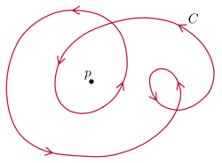
One can also consider the winding number of the path with respect to the tangent of the path itself. As a path followed through time, this would be the winding number with respect to the origin of the velocity vector. In this case the example illustrated at the beginning of this article has a winding number of 3, because the small loop is counted.
This is only defined for immersed paths (i.e., for differentiable paths with nowhere vanishing derivatives), and is the degree of the tangential Gauss map.
This is called the turning number, and can be computed as the total curvature divided by 2π.
Winding number and Heisenberg ferromagnet equations
The winding number is closely related with the (2 + 1)-dimensional continuous Heisenberg ferromagnet equations and its integrable extensions: the Ishimori equation etc. Solutions of the last equations are classified by the winding number or topological charge (topological invariant and/or topological quantum number).
See also
- Argument principle
- Linking coefficient
- Nonzero-rule
- Polygon density
- Residue theorem
- Topological degree theory
- Topological quantum number
- Wilson loop
- Writhe
References
- Möbius, August (1865). "Über die Bestimmung des Inhaltes eines Polyëders". Berichte über die Verhandlungen der Königlich Sächsischen Gesellschaft der Wissenschaften, Mathematisch-Physische Klasse. 17: 31–68.
- Alexander, J. W. (April 1928). "Topological Invariants of Knots and Links". Transactions of the American Mathematical Society. 30 (2): 275–306. doi:10.2307/1989123.
- Weisstein, Eric W. "Contour Winding Number." From MathWorld--A Wolfram Web Resource. http://mathworld.wolfram.com/ContourWindingNumber.html
- Rudin, Walter (1976). Principles of Mathematical Analysis. New York: McGraw-Hill. p. 201. ISBN 0-07-054235-X.
- Rudin, Walter (1987). Real and Complex Analysis (3rd ed.). New York: McGraw-Hill. p. 203. ISBN 0-07-054234-1.
External links
- "Winding number". PlanetMath.