Ray tracing (graphics)

On input we have (in calculation we use vector normalization and cross product):

• ${\displaystyle E\in \mathbb {R^{3}} }$ eye position
• ${\displaystyle T\in \mathbb {R^{3}} }$ target position
• ${\displaystyle \theta \in [0,\pi ]}$ field of view - for human we can assume ${\displaystyle \approx \pi /2{\text{ rad}}=90^{\circ }}$
• ${\displaystyle m,k\in \mathbb {N} }$ numbers of square pixels on viewport vertical and horizontal direction
• ${\displaystyle i,j\in \mathbb {N} ,1\leq i\leq k\land 1\leq j\leq m}$ numbers of actual pixel
• ${\displaystyle {\vec {w}}\in \mathbb {R^{3}} }$ vertical vector which indicates where is up and down, usually ${\displaystyle {\vec {w}}=[0,1,0]}$ (not visible on picture) - roll component which determine viewport rotation around point C (where the axis of rotation is the ET section)

The idea is to find the position of each viewport pixel center ${\displaystyle P_{ij}}$ which allows us to find the line going from eye ${\displaystyle E}$ through that pixel and finally get the ray described by point ${\displaystyle E}$ and vector ${\displaystyle {\vec {R}}_{ij}=P_{ij}-E}$ (or its normalisation ${\displaystyle {\vec {r}}_{ij}}$). First we need to find the coordinates of the bottom left viewport pixel ${\displaystyle P_{1m}}$ and find the next pixel by making a shift along directions parallel to viewport (vectors ${\displaystyle {\vec {b}}_{n}}$ i ${\displaystyle {\vec {v}}_{n}}$) multiplied by the size of the pixel. Below we introduce formulas which include distance ${\displaystyle d}$ between the eye and the viewport. However, this value will be reduced during ray normalization ${\displaystyle {\vec {r}}_{ij}}$ (so you might as well accept that ${\displaystyle d=1}$ and remove it from calculations).

Pre-calculations: let's find and normalise vector ${\displaystyle {\vec {t}}}$ and vectors ${\displaystyle {\vec {b}},{\vec {v}}}$ which are parallel to the viewport (all depicted on above picture)

${\displaystyle {\vec {t}}=T-E,\qquad {\vec {b}}={\vec {w}}\times {\vec {t}}}$

${\displaystyle {\vec {t}}_{n}={\frac {\vec {t}}{||{\vec {t}}||}},\qquad {\vec {b}}_{n}={\frac {\vec {b}}{||{\vec {b}}||}},\qquad {\vec {v}}_{n}={\vec {t}}_{n}\times {\vec {b}}_{n}}$

note that viewport center ${\displaystyle C=E+{\vec {t}}_{n}d}$, next we calculate viewport sizes ${\displaystyle h_{x},h_{y}}$ divided by 2 including aspect ratio ${\displaystyle {\frac {m}{k}}}$

${\displaystyle g_{x}={\frac {h_{x}}{2}}=d\tan {\frac {\theta }{2}},\qquad g_{y}={\frac {h_{y}}{2}}=g_{x}{\frac {m}{k}}}$

and then we calculate next-pixel shifting vectors ${\displaystyle q_{x},q_{y}}$ along directions parallel to viewport (${\displaystyle {\vec {b}},{\vec {v}}}$), and left bottom pixel center ${\displaystyle p_{1m}}$

${\displaystyle {\vec {q}}_{x}={\frac {2g_{x}}{k-1}}{\vec {b}}_{n},\qquad {\vec {q}}_{y}={\frac {2g_{y}}{m-1}}{\vec {v}}_{n},\qquad {\vec {p}}_{1m}={\vec {t}}_{n}d-g_{x}{\vec {b}}_{n}-g_{y}{\vec {v}}_{n}}$

Calculations: note ${\displaystyle P_{ij}=E+{\vec {p}}_{ij}}$ and ray ${\displaystyle {\vec {R}}_{ij}=P_{ij}-E={\vec {p}}_{ij}}$ so

${\displaystyle {\vec {p}}_{ij}={\vec {p}}_{1m}+{\vec {q}}_{x}(i-1)+{\vec {q}}_{y}(j-1)}$

${\displaystyle {\vec {r}}_{ij}={\frac {{\vec {R}}_{ij}}{||{\vec {R}}_{ij}||}}={\frac {{\vec {p}}_{ij}}{||{\vec {p}}_{ij}||}}}$

Above formula was tested in this javascript project (works in browser).

In nature, a light source emits a ray of light which travels, eventually, to a surface that interrupts its progress. One can think of this "ray" as a stream of photons traveling along the same path. In a perfect vacuum this ray will be a straight line (ignoring relativistic effects). Any combination of four things might happen with this light ray: absorption, reflection, refraction and fluorescence. A surface may absorb part of the light ray, resulting in a loss of intensity of the reflected and/or refracted light. It might also reflect all or part of the light ray, in one or more directions. If the surface has any transparent or translucent properties, it refracts a portion of the light beam into itself in a different direction while absorbing some (or all) of the spectrum (and possibly altering the color). Less commonly, a surface may absorb some portion of the light and fluorescently re-emit the light at a longer wavelength color in a random direction, though this is rare enough that it can be discounted from most rendering applications. Between absorption, reflection, refraction and fluorescence, all of the incoming light must be accounted for, and no more. A surface cannot, for instance, reflect 66% of an incoming light ray, and refract 50%, since the two would add up to be 116%. From here, the reflected and/or refracted rays may strike other surfaces, where their absorptive, refractive, reflective and fluorescent properties again affect the progress of the incoming rays. Some of these rays travel in such a way that they hit our eye, causing us to see the scene and so contribute to the final rendered image.

The first ray tracing algorithm used for rendering was presented by Arthur Appel in 1968.[2] This algorithm has since been termed "ray casting". The idea behind ray casting is to trace rays from the eye, one per pixel, and find the closest object blocking the path of that ray. Think of an image as a screen-door, with each square in the screen being a pixel. This is then the object the eye sees through that pixel. Using the material properties and the effect of the lights in the scene, this algorithm can determine the shading of this object. The simplifying assumption is made that if a surface faces a light, the light will reach that surface and not be blocked or in shadow. The shading of the surface is computed using traditional 3D computer graphics shading models. One important advantage ray casting offered over older scanline algorithms was its ability to easily deal with non-planar surfaces and solids, such as cones and spheres. If a mathematical surface can be intersected by a ray, it can be rendered using ray casting. Elaborate objects can be created by using solid modeling techniques and easily rendered.

Ray tracing can create realistic-looking images.

In addition to the high degree of realism, ray tracing can simulate the effects of a camera due to depth of field and aperture shape (in this case a hexagon).

The number of reflections, or bounces, a “ray” can make, and how it is affected each time it encounters a surface, is controlled by settings in the software. In this image, each ray was allowed to reflect up to 16 times. Multiple “reflections of reflections” can thus be seen in these spheres. (Image created with Cobalt.)

The number of refractions a “ray” can make, and how it is affected each time it encounters a surface that permits the transmission of light, is controlled by settings in the software. Here, each ray was set to refract or reflect (the "depth") up to 9 times. Fresnel reflections were used and caustics are visible. (Image created with V-Ray.)

The next important research breakthrough came from Turner Whitted in 1979.[3] Previous algorithms traced rays from the eye into the scene until they hit an object, but determined the ray color without recursively tracing more rays. Whitted continued the process. When a ray hits a surface, it can generate up to three new types of rays: reflection, refraction, and shadow.[4] A reflection ray is traced in the mirror-reflection direction. The closest object it intersects is what will be seen in the reflection. Refraction rays traveling through transparent material work similarly, with the addition that a refractive ray could be entering or exiting a material. A shadow ray is traced toward each light. If any opaque object is found between the surface and the light, the surface is in shadow and the light does not illuminate it. This recursive ray tracing added more realism to ray traced images.

Ray tracing-based rendering's popularity stems from its basis in a realistic simulation of light transport, as compared to other rendering methods, such as rasterization, which focuses more on the realistic simulation of geometry. Effects such as reflections and shadows, which are difficult to simulate using other algorithms, are a natural result of the ray tracing algorithm. The computational independence of each ray makes ray tracing amenable to a basic level of parallelization,[5][6] but the divergence of ray paths makes high utilization under parallelism quite difficult to achieve in practice.[7]

A serious disadvantage of ray tracing is performance (though it can in theory be faster than traditional scanline rendering depending on scene complexity vs. number of pixels on-screen). Until the late 2010s, ray tracing in real time was usually considered impossible on consumer hardware for nontrivial tasks. Scanline algorithms and other algorithms use data coherence to share computations between pixels, while ray tracing normally starts the process anew, treating each eye ray separately. However, this separation offers other advantages, such as the ability to shoot more rays as needed to perform spatial anti-aliasing and improve image quality where needed.

Although it does handle interreflection and optical effects such as refraction accurately, traditional ray tracing is also not necessarily photorealistic. True photorealism occurs when the rendering equation is closely approximated or fully implemented. Implementing the rendering equation gives true photorealism, as the equation describes every physical effect of light flow. However, this is usually infeasible given the computing resources required.

The realism of all rendering methods can be evaluated as an approximation to the equation. Ray tracing, if it is limited to Whitted's algorithm, is not necessarily the most realistic. Methods that trace rays, but include additional techniques (photon mapping, path tracing), give a far more accurate simulation of real-world lighting.

The process of shooting rays from the eye to the light source to render an image is sometimes called backwards ray tracing, since it is the opposite direction photons actually travel. However, there is confusion with this terminology. Early ray tracing was always done from the eye, and early researchers such as James Arvo used the term backwards ray tracing to mean shooting rays from the lights and gathering the results. Therefore, it is clearer to distinguish eye-based versus light-based ray tracing.

While the direct illumination is generally best sampled using eye-based ray tracing, certain indirect effects can benefit from rays generated from the lights. Caustics are bright patterns caused by the focusing of light off a wide reflective region onto a narrow area of (near-)diffuse surface. An algorithm that casts rays directly from lights onto reflective objects, tracing their paths to the eye, will better sample this phenomenon. This integration of eye-based and light-based rays is often expressed as bidirectional path tracing, in which paths are traced from both the eye and lights, and the paths subsequently joined by a connecting ray after some length.[8][9]

Photon mapping is another method that uses both light-based and eye-based ray tracing; in an initial pass, energetic photons are traced along rays from the light source so as to compute an estimate of radiant flux as a function of 3-dimensional space (the eponymous photon map itself). In a subsequent pass, rays are traced from the eye into the scene to determine the visible surfaces, and the photon map is used to estimate the illumination at the visible surface points.[10][11] The advantage of photon mapping versus bidirectional path tracing is the ability to achieve significant reuse of photons, reducing computation, at the cost of statistical bias.

An additional problem occurs when light must pass through a very narrow aperture to illuminate the scene (consider a darkened room, with a door slightly ajar leading to a brightly lit room), or a scene in which most points do not have direct line-of-sight to any light source (such as with ceiling-directed light fixtures or torchieres). In such cases, only a very small subset of paths will transport energy; Metropolis light transport is a method which begins with a random search of the path space, and when energetic paths are found, reuses this information by exploring the nearby space of rays.[12]

Image showing recursively generated rays from the "eye" (and through an image plane) to a light source after encountering two diffuse surfaces.

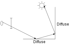
To the right is an image showing a simple example of a path of rays recursively generated from the camera (or eye) to the light source using the above algorithm. A diffuse surface reflects light in all directions.

First, a ray is created at an eyepoint and traced through a pixel and into the scene, where it hits a diffuse surface. From that surface the algorithm recursively generates a reflection ray, which is traced through the scene, where it hits another diffuse surface. Finally, another reflection ray is generated and traced through the scene, where it hits the light source and is absorbed. The color of the pixel now depends on the colors of the first and second diffuse surface and the color of the light emitted from the light source. For example, if the light source emitted white light and the two diffuse surfaces were blue, then the resulting color of the pixel is blue.

As a demonstration of the principles involved in ray tracing, consider how one would find the intersection between a ray and a sphere. This is merely the math behind the line–sphere intersection and the subsequent determination of the colour of the pixel being calculated. There is, of course, far more to the general process of ray tracing, but this demonstrates an example of the algorithms used.

In vector notation, the equation of a sphere with center ${\displaystyle \mathbf {c} }$ and radius ${\displaystyle r}$ is

${\displaystyle \left\Vert \mathbf {x} -\mathbf {c} \right\Vert ^{2}=r^{2}.}$

Any point on a ray starting from point ${\displaystyle \mathbf {s} }$ with direction ${\displaystyle \mathbf {d} }$ (here ${\displaystyle \mathbf {d} }$ is a unit vector) can be written as

${\displaystyle \mathbf {x} =\mathbf {s} +t\mathbf {d} ,}$

where ${\displaystyle t}$ is its distance between ${\displaystyle \mathbf {x} }$ and ${\displaystyle \mathbf {s} }$. In our problem, we know ${\displaystyle \mathbf {c} }$, ${\displaystyle r}$, ${\displaystyle \mathbf {s} }$ (e.g. the position of a light source) and ${\displaystyle \mathbf {d} }$, and we need to find ${\displaystyle t}$. Therefore, we substitute for ${\displaystyle \mathbf {x} }$:

${\displaystyle \left\Vert \mathbf {s} +t\mathbf {d} -\mathbf {c} \right\Vert ^{2}=r^{2}.}$

Let ${\displaystyle \mathbf {v} \ {\stackrel {\mathrm {def} }{=}}\ \mathbf {s} -\mathbf {c} }$ for simplicity; then

${\displaystyle \left\Vert \mathbf {v} +t\mathbf {d} \right\Vert ^{2}=r^{2}}$

${\displaystyle \mathbf {v} ^{2}+t^{2}\mathbf {d} ^{2}+2\mathbf {v} \cdot t\mathbf {d} =r^{2}}$

${\displaystyle (\mathbf {d} ^{2})t^{2}+(2\mathbf {v} \cdot \mathbf {d} )t+(\mathbf {v} ^{2}-r^{2})=0.}$

Knowing that d is a unit vector allows us this minor simplification:

${\displaystyle t^{2}+(2\mathbf {v} \cdot \mathbf {d} )t+(\mathbf {v} ^{2}-r^{2})=0.}$

This quadratic equation has solutions

${\displaystyle t={\frac {-(2\mathbf {v} \cdot \mathbf {d} )\pm {\sqrt {(2\mathbf {v} \cdot \mathbf {d} )^{2}-4(\mathbf {v} ^{2}-r^{2})}}}{2}}=-(\mathbf {v} \cdot \mathbf {d} )\pm {\sqrt {(\mathbf {v} \cdot \mathbf {d} )^{2}-(\mathbf {v} ^{2}-r^{2})}}.}$

The two values of ${\displaystyle t}$ found by solving this equation are the two ones such that ${\displaystyle \mathbf {s} +t\mathbf {d} }$ are the points where the ray intersects the sphere.

Any value which is negative does not lie on the ray, but rather in the opposite half-line (i.e. the one starting from ${\displaystyle \mathbf {s} }$ with opposite direction).

If the quantity under the square root ( the discriminant ) is negative, then the ray does not intersect the sphere.

Let us suppose now that there is at least a positive solution, and let ${\displaystyle t}$ be the minimal one. In addition, let us suppose that the sphere is the nearest object on our scene intersecting our ray, and that it is made of a reflective material. We need to find in which direction the light ray is reflected. The laws of reflection state that the angle of reflection is equal and opposite to the angle of incidence between the incident ray and the normal to the sphere.

The normal to the sphere is simply

${\displaystyle \mathbf {n} ={\frac {\mathbf {y} -\mathbf {c} }{\left\Vert \mathbf {y} -\mathbf {c} \right\Vert }},}$

where ${\displaystyle \mathbf {y} =\mathbf {s} +t\mathbf {d} }$ is the intersection point found before. The reflection direction can be found by a reflection of ${\displaystyle \mathbf {d} }$ with respect to ${\displaystyle \mathbf {n} }$, that is

${\displaystyle \mathbf {r} =\mathbf {d} -2(\mathbf {n} \cdot \mathbf {d} )\mathbf {n} .}$

Thus the reflected ray has equation

${\displaystyle \mathbf {x} =\mathbf {y} +u\mathbf {r} .\,}$

Now we only need to compute the intersection of the latter ray with our field of view, to get the pixel which our reflected light ray will hit. Lastly, this pixel is set to an appropriate color, taking into account how the color of the original light source and the one of the sphere are combined by the reflection.

References

- Georg Rainer Hofmann (1990). "Who invented ray tracing?". The Visual Computer. 6 (3): 120–124. doi:10.1007/BF01911003..
- Appel A. (1968) Some techniques for shading machine renderings of solids. AFIPS Conference Proc. 32 pp.37-45
- Whitted T. (1979) An improved illumination model for shaded display. Proceedings of the 6th annual conference on Computer graphics and interactive techniques
- Tomas Nikodym (June 2010). "Ray Tracing Algorithm For Interactive Applications" (PDF). Czech Technical University, FEE.
- J.-C. Nebel. A New Parallel Algorithm Provided by a Computation Time Model, Eurographics Workshop on Parallel Graphics and Visualisation, 24–25 September 1998, Rennes, France.
- A. Chalmers, T. Davis, and E. Reinhard. Practical parallel rendering, ISBN 1-56881-179-9. AK Peters, Ltd., 2002.
- Aila, Timo and Samulii Laine, Understanding the Efficiency of Ray Traversal on GPUs, High Performance Graphics 2009, New Orleans, LA.
- Eric P. Lafortune and Yves D. Willems (December 1993). "Bi-Directional Path Tracing". Proceedings of Compugraphics '93: 145–153.
- Péter Dornbach. "Implementation of bidirectional ray tracing algorithm". Retrieved June 11, 2008.
- Global Illumination using Photon Maps Archived 2008-08-08 at the Wayback Machine
- Photon Mapping - Zack Waters
- http://graphics.stanford.edu/papers/metro/metro.pdf
- Hall, Roy A.; Greenberg, Donald P. (November 1983). "A Testbed for Realistic Image Synthesis". IEEE Computer Graphics and Applications. 3 (8): 10–20. CiteSeerX 10.1.1.131.1958. doi:10.1109/MCG.1983.263292.
- "【Osaka University 】 LINKS-1 Computer Graphics System". IPSJ Computer Museum. Information Processing Society of Japan. Retrieved November 15, 2018.
- Defanti, Thomas A. (1984). Advances in computers. Volume 23 (PDF). Academic Press. p. 121. ISBN 0-12-012123-9.
- See Proceedings of 4th Computer Graphics Workshop, Cambridge, MA, USA, October 1987. Usenix Association, 1987. pp 86–98.
- "About BRL-CAD". Retrieved January 18, 2019.
- Piero Foscari. "The Realtime Raytracing Realm". ACM Transactions on Graphics. Retrieved September 17, 2007.
- Parker, Steven; Martin, William (April 26, 1999). "Interactive ray tracing". I3D '99 Proceedings of the 1999 Symposium on Interactive 3D Graphics (April 1999): 119–126. CiteSeerX 10.1.1.6.8426. doi:10.1145/300523.300537. ISBN 1581130821. Retrieved October 30, 2019.
- Mark Ward (March 16, 2007). "Rays light up life-like graphics". BBC News. Retrieved September 17, 2007.
- Theo Valich (June 12, 2008). "Intel converts ET: Quake Wars to ray tracing". TG Daily. Retrieved June 16, 2008.
- Nvidia (October 18, 2009). "Nvidia OptiX". Nvidia. Retrieved November 6, 2009.
- "3DWorld: Hardware review: Caustic Series2 R2500 ray-tracing accelerator card". Retrieved April 23, 2013.3D World, April 2013
- Cuthbert, Dylan (October 24, 2015). "Creating the beautiful, ground-breaking visuals of The Tomorrow Children on PS4". PlayStation Blog. Retrieved December 7, 2015.
- GPUOpen Real-time Ray-tracing
- James, Dave (June 11, 2019). "AMD's second-gen RDNA GPUs will feature hardware-accelerated ray tracing in 2020". PCGamesN. Retrieved June 14, 2019.
- Warren, Tom (June 8, 2019). "Microsoft hints at next-generation Xbox 'Scarlet' in E3 teasers". The Verge. Retrieved October 8, 2019.
- Chaim, Gartenberg (October 8, 2019). "Sony confirms PlayStation 5 name, holiday 2020 release date". The Verge. Retrieved October 8, 2019.
- Warren, Tom (February 24, 2020). "Microsoft reveals more Xbox Series X specs, confirms 12 teraflops GPU". The Verge. Retrieved February 25, 2020.
- "Computability and Complexity of Ray Tracing". https://www.cs.duke.edu/~reif/paper/tygar/raytracing.pdf